Machine Learning Algorithm Evaluation
Because Ghost blogs recognize LateX syntax differently from standard LateX syntax, the LateX formulas in the following article may appear garbled for better generality. If they do, and you do not mind, you can read the garble-free version of this article on the author’s Github. The author will fix this garbling issue when time permits. Thank you for your understanding.
GitHub Repo: Halfrost-Field
Follow: halfrost · GitHub
Source: https://github.com/halfrost/Halfrost-Field/blob/master/contents/Machine_Learning/Advice_for_Applying_Machine_Learning.ipynb
I. Evaluating a Learning Algorithm
To reduce prediction error—that is, to improve prediction accuracy—we often use the following approaches:
Collect more samples
It is a mistake to assume that more samples are always better; in fact, more data is not necessarily better.Reduce feature dimensionality
Dimensionality reduction may remove useful features.Collect more features
This increases the computational burden and may also lead to overfitting.Perform higher-order polynomial regression
An overly high-order polynomial may cause overfitting.Tune the regularization parameter $\lambda$, increasing or decreasing $\lambda$
Increasing or decreasing it is often done by intuition.
With so many possible solutions, how do we know which one to choose? Many people choose one of these methods purely by intuition, spend a long time on it, and eventually discover it is useless—going down a dead end. Therefore, below we introduce a simple and effective approach that we call a machine learning diagnostic.
1. Evaluating a Hypothesis
The first thing we need to evaluate is our hypothesis. When we choose feature values or parameters to minimize the training-set error, we may encounter overfitting, and the model will no longer work well when generalized to new data. Moreover, when there are many features, we cannot visualize $J(\theta)$ to see whether it decreases as the number of iterations increases. Therefore, we use the following method to evaluate our hypothesis:
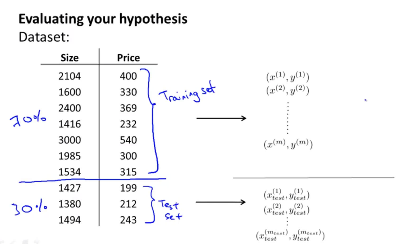
Suppose there are 10 data points. Randomly use 70% as the training set and the remaining 30% as the test set. Try to ensure that the training set and test set are randomly shuffled.
Next:
- Learn the parameters $\Theta$ from the training set; that is, use the training set to minimize the training error $J_{train}(\Theta)$
- Compute the test error $J_{test}(\Theta)$ by taking the parameters $\Theta$ learned from the training set and using them here to compute the test error.
For linear regression: $$J_{test}(\theta)=\frac{1}{2m_{test}}\sum_{i=1}^{m_{test}}{(h_\theta(x^{(i)}_{test})-y^{(i)}_{test})^2}$$
For logistic regression: $$J_{test}(\theta)=-\frac{1}{m_{test}}\sum_{i=1}^{m_{test}}{y^{(i)}_{test}logh_\theta(x^{(i)}_{test})+(1-y^{(i)}_{test})logh_\theta(x^{(i)}_{test})}$$
Logistic regression differs from linear regression because it has only two values, 0 and 1. Therefore, the error is determined as follows:
$$ err(h_\theta(x),y)=\left{\begin{matrix} 1 ;;;( if ;;; h_\theta(x) \geqslant 0.5 , y=0 ;;;or;;; if;;; h_\theta(x) < 0.5 , y=1 )\ 0 ;;;( otherwise ) ;;;;;;;;;;;;;;;;;;;;;;;;;;;;;;;;;;;;;;;;;;;;;;;;;;;;; \end{matrix}\right. $$
The error here is also called the misclassification rate, or the $0/1$ misclassification rate.
$( if ;;; h_\theta(x) \geqslant 0.5 , y=0 ;;;or;;; if;;; h_\theta(x) < 0.5 , y=1 )$
In this case, the hypothesis result is more inclined toward 1, but the actual label is 0; or the hypothesis result is more inclined toward 0, but the actual label is 1.
If none of the above cases occur, then there is no error, i.e., it is 0, which also means that the hypothesis value can correctly classify the sample.
The average test error on the test set is:
$$Test;Error=\frac{1}{m_{test}}\sum_{i=1}^{m_{test}}err(h_{\theta}(x^{(i)}_{test}),y^{(i)}_{test})$$
2. Model Selection and Train/Validation/Test Sets
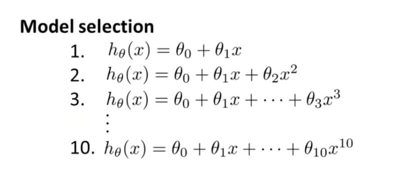
Here we use d to denote the number of polynomial terms. We can change the degree of the polynomial to choose a model that suits our data. For example, in the above $h_\theta(x)=\theta_0+\theta_1x$ , this polynomial has $d=1$ .
We can test each model to obtain its $J_{test}(\theta)$ and determine which model is better.
Once we have selected a polynomial degree d that fits the test set perfectly, we can no longer use the test set, because d has already been chosen to perfectly fit the test set; testing on it again is meaningless. We need a different test set. What we should care about more is how well it fits new samples.
To solve the problem above, we divide the data into 3 sets: 60% training set / 20% cross-validation set / 20% test set.
Using these three sets, we can compute the training error:
$$J_{train}(\theta) = \frac{1}{2m}\sum_{i=1}^{m}(h_\theta(x^{(i)})-y^{(i)})^{2}$$
Cross-validation error:
$$J_{cv}(\theta) = \frac{1}{2m_{cv}}\sum_{i=1}^{m_{cv}}(h_\theta(x^{(i)}_{cv})-y^{(i)}_{cv})^{2}$$
Test error:
$$J_{test}(\theta) = \frac{1}{2m_{test}}\sum_{i=1}^{m}(h_\theta(x^{(i)}_{test})-y^{(i)}_{test})^{2}$$
Thus, we no longer select a model solely based on the test set. Instead:
- Use the training-set data with each polynomial model.
- Use the cross-validation-set data to find the polynomial model with the minimum error.
- Finally, use the test set to find the model with relatively smaller error.
II. Bias vs. Variance
1. Diagnosing Bias vs. Variance
In machine learning, bias reflects the model’s inability to capture the patterns in the data, while variance reflects that the model is overly sensitive to the training set and loses the underlying data patterns. Both high bias and high variance can cause the model to make incorrect predictions when new data arrives.
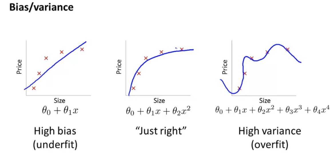
Still using this figure as an example, the leftmost plot shows underfitting, and the rightmost plot shows overfitting.
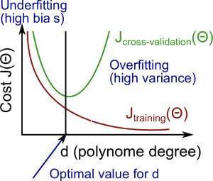
The figure above shows how the training-set and cross-validation-set errors vary with the polynomial degree d. The horizontal axis is our d, i.e., the number of polynomial terms, and the vertical axis is our cost function.
First, let’s look at the red curve $J_{training}(\theta)$ . As the number of polynomial terms increases, the hypothesis function gets closer and closer to the data to be fitted, so its cost function decreases as the number of polynomial terms increases.
The green curve is $J_{cross-validation}(\theta)$ . When the number of polynomial terms is small, underfitting naturally occurs, so initially its cost function $J_{cross-validation}(\theta)$ is very large and decreases as the number of polynomial terms increases. However, if the number of polynomial terms continues to increase, overfitting occurs, and $J_{cross-validation}(\theta)$ increases again. Therefore, the $J_{cross-validation}(\theta)$ function first decreases and then increases; its lowest point corresponds to the most appropriate polynomial degree.
In polynomial regression, if the polynomial degree is high, overfitting is likely to occur. At this point, the training error is very low, but the generalization ability on new data is poor, causing the errors on both the cross-validation set and the test set to be high. In this case, the model exhibits high variance (overfitting):
$$ \left{\begin{matrix} J_{train}(\theta) ;;;is;; low\ J_{cv}(\theta)»J_{test}(\theta) \end{matrix}\right. $$
In the case of overfitting, the training-set error is usually small and much smaller than the cross-validation error.
When the degree is low, underfitting is likely to occur. At this point, the training set, cross-validation set, and test set all have high error. In this case, the model exhibits high bias (underfitting):
$$ \left{\begin{matrix} J_{train}(\theta),J_{cv}(\theta);;; is ;; high\ J_{cv}(\theta) \approx J_{test}(\theta) \end{matrix}\right. $$
In the case of underfitting, the training-set error will be large.
Why does $J_{cross-validation}(\theta)$ first decrease and then increase, while $J_{training}(\theta)$ keeps decreasing?
The reason is that $\theta$ is trained only on the training set. When it is substituted into $J_{cross-validation}(\theta)$, as the polynomial degree increases, the data deviation becomes larger and larger.
2. Regularization and Bias/Variance: Bias and Variance in Regularization
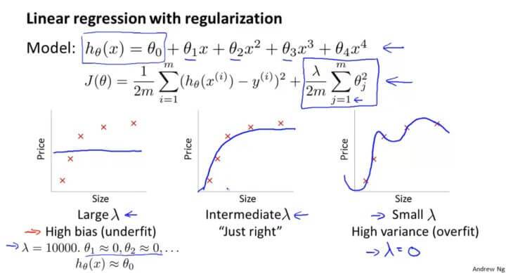
To prevent overfitting, we add a regularization term. But what is the relationship between the regularization parameter $\lambda$ and overfitting?
When $\lambda$ is very large, every subsequent $\theta_i$ is penalized, leaving only $\theta_0$. The hypothesis function then becomes a straight line, resulting in underfitting.
When $\lambda$ is very small, an extreme example is $\lambda=0$, which is equivalent to not adding the regularization term at all. This leads to overfitting.
The value of $\lambda$ should be neither too large nor too small.
The value of $\lambda$ can be chosen from $\left[0,0.01,0.02,0.04,0.08,0.16,0.32,0.64,1.28,2.56,5.12,10.24\right]$. For each of the 12 different models, compute the minimum cost function for each value of $\lambda$, thereby obtaining $\Theta^{(i)}$.
After obtaining the 12 $\Theta^{(i)}$ values, evaluate them using the cross-validation set. That is, compute the average squared error $J_{cv}(\Theta^{(i)})$ for each $\Theta$ on the cross-validation set.
Choose the $\lambda$ with the smallest cross-validation error—the one that best fits the data—as the regularization parameter.
Finally, use this regularization parameter on the test set to evaluate how well $J_{test}(\Theta^{(i)})$ predicts.
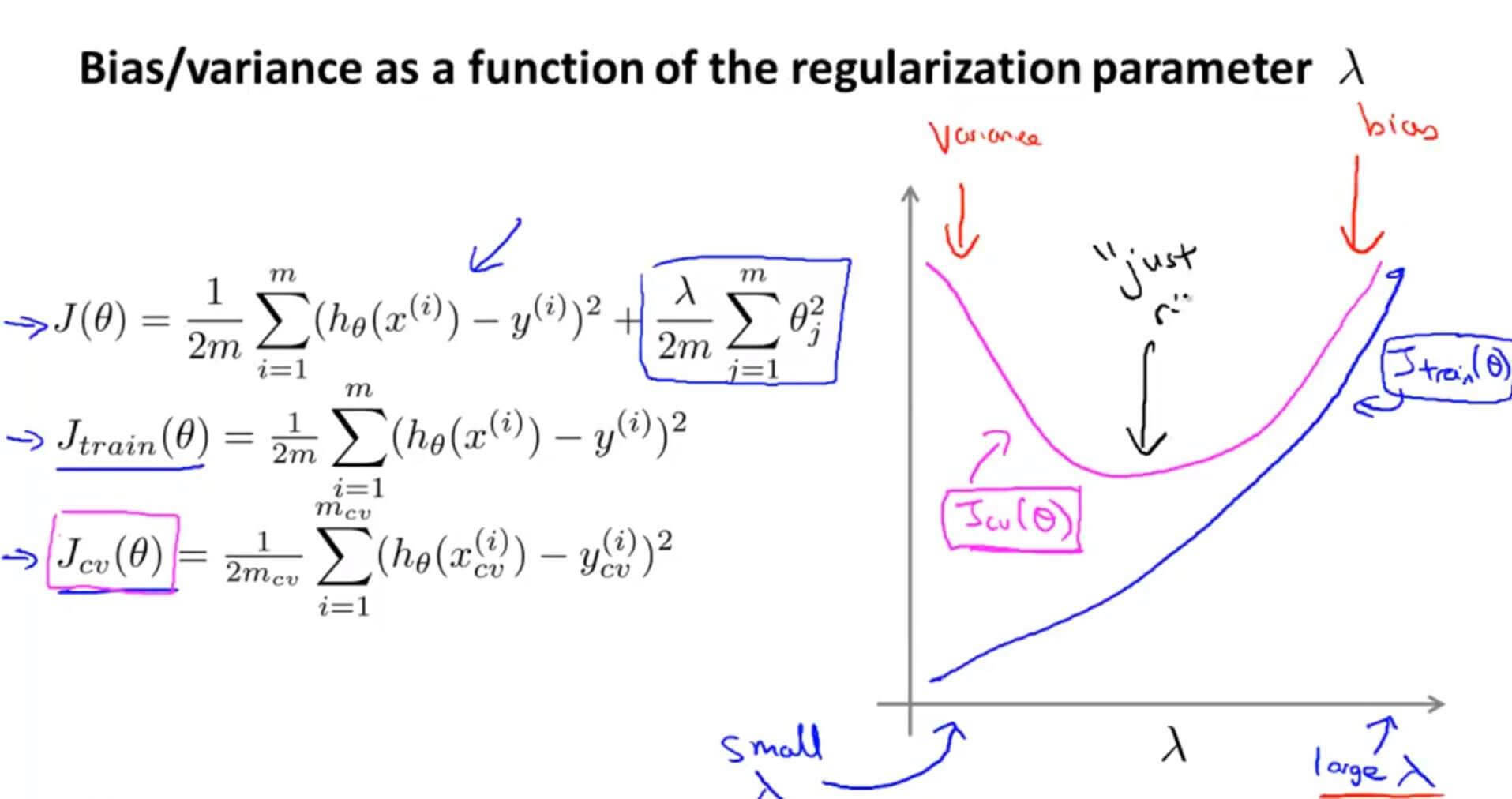
As the parameter $\lambda$ increases, $J_{train}(\theta)$ naturally increases as well. This is because when $\lambda=0$, $J_{train}(\theta)$ has no regularization term.
But for $J_{cv}(\theta)$, the $\theta$ in the hypothesis function is fitted from the training set, so before regularization is added, $J_{cv}(\theta)$ is very large. As $\lambda$ gradually increases—that is, as the effect of regularization gradually becomes apparent—the model fits the cross-validation and test data better and better, so $J_{cv}(\theta)$ naturally decreases. However, when $\lambda$ becomes sufficiently large, $h_\theta(x)$ for the cross-validation set will approach a straight line, and $J_{cv}(\theta)$ will naturally rise again.
3. Learning Curves
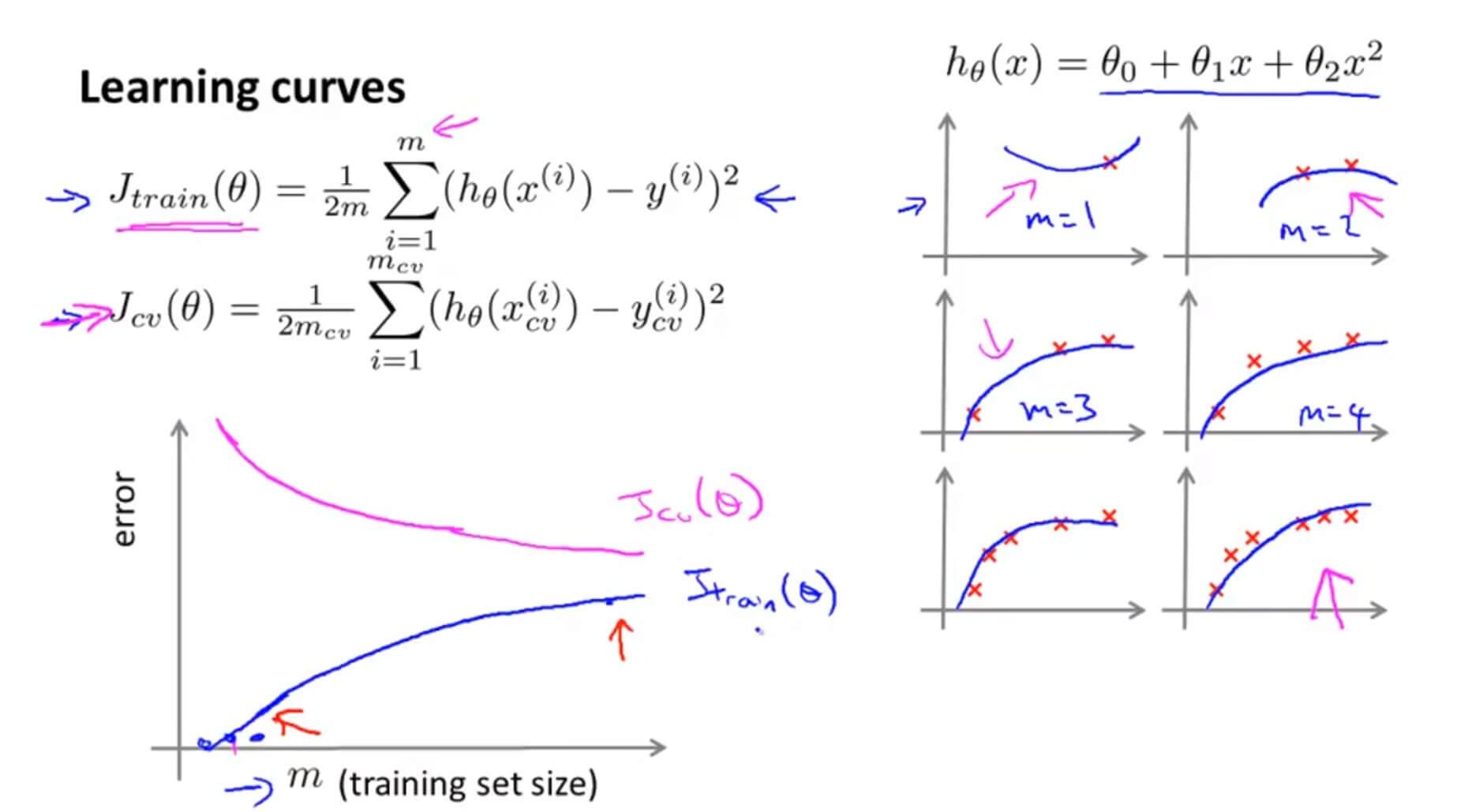
Suppose we use $h_\theta(x)=\theta_0+\theta_1x+\theta_2x^2$ to fit the data. When there are only a few data points, the fit is of course very good. However, as the amount of data increases, our hypothesis function cannot fit the data well because the polynomial has too few terms. Therefore, the training error $J_{train}(\theta)$ increases as the amount of data increases, as shown by the blue curve in the figure above.
What about the cross-validation set? Since there are only a few data points at the beginning, the parameters fitted on the training set are very likely not suitable for the cross-validation set, so the error is large when the data size is small. But as the amount of data gradually increases, even though some individual data points cannot be fitted well, the overall fit is certainly better than when there were only a few data points, so the overall error gradually decreases, as shown by the pink curve in the figure above.
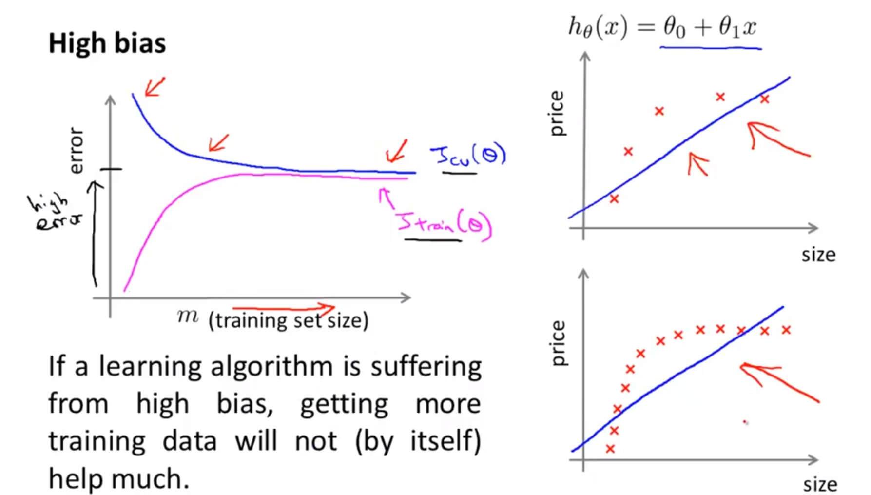
When the data has high bias, that is, underfitting, adding more data will not help. Therefore, the error will converge to an equilibrium point, and both $J_{train}(\theta)$ and $J_{cv}(\theta)$ will have large errors.
So, when the data has an underfitting problem, using more training examples cannot solve it.
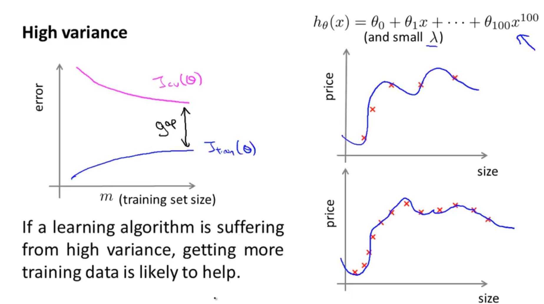
When the data has high variance, that is, overfitting, as the amount of data increases, the model can still fit the training data almost perfectly because it is overfitting. Therefore, although the training error increases, it does so very slowly; the same applies to the cross-validation set. Thus, when overfitting occurs, the curve looks like the figure above, with a large gap between $J_{train}(\theta)$ and $J_{cv}(\theta)$.
So, when the data has an overfitting problem, using more examples helps us solve it.
4. Deciding What to Do Next Revisited
Summary:
| Method | When to Use |
|---|---|
| Collect more examples | High variance (overfitting) |
| Reduce feature dimensionality | High variance (overfitting) |
| Collect more features | High bias (underfitting) |
| Use higher-degree polynomial regression | High bias (underfitting) |
| Decrease parameter λ | High bias (underfitting) |
| Increase parameter λ | High variance (overfitting) |
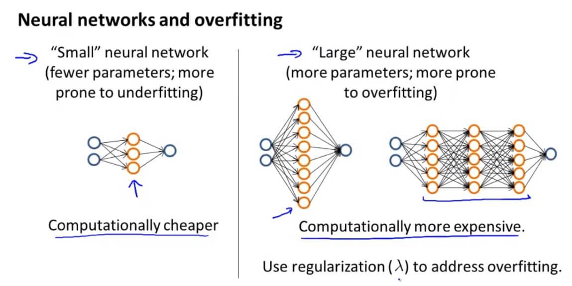
When we choose relatively small neural networks, they require less computation, but they are prone to underfitting. Conversely, if we choose neural networks with more layers and more units per layer, they are prone to overfitting. We mentioned earlier that larger neural networks tend to perform better. To prevent overfitting, we can apply regularization.
Using a single hidden layer is a good default starting point. You can train your neural network with different numbers of hidden layers using the cross-validation set. Then you can choose the one with the best performance.
Impact of model complexity:
- Low-degree polynomials (low model complexity) have high bias and low variance. In this case, the model has difficulty fitting the data consistently.
- High-degree polynomials (high model complexity) fit the training data very well but perform extremely poorly on test data. They have low bias on the training data but high variance.
- In practice, we want to choose a model somewhere between the two: one that generalizes well while still fitting the data well.
III. Advice for Applying Machine Learning: Quiz
1. Question 1
You train a learning algorithm, and find that it has unacceptably high error on the test set. You plot the learning curve, and obtain the figure below. Is the algorithm suffering from high bias, high variance, or neither?

A. High variance
B. Neither
C. High bias
Answer: A
This is the curve for high variance.
2. Question 2
Suppose you have implemented regularized logistic regression to classify what object is in an image (i.e., to do object recognition). However, when you test your hypothesis on a new set of images, you find that it makes unacceptably large errors with its predictions on the new images. However, your hypothesis performs well (has low error) on the training set. Which of the following are promising steps to take? Check all that apply.
A. Try adding polynomial features.
B. Get more training examples.
C. Try using a smaller set of features.
D. Use fewer training examples.
Answer: B, C
For overfitting, you can reduce the number of features, increase the number of training examples, or increase the regularization parameter $\lambda$.
3. Question 3
Suppose you have implemented regularized logistic regression to predict what items customers will purchase on a web shopping site. However, when you test your hypothesis on a new set of customers, you find that it makes unacceptably large errors in its predictions. Furthermore, the hypothesis performs poorly on the training set. Which of the following might be promising steps to take? Check all that apply.
A. Try using a smaller set of features.
B. Try adding polynomial features.
C. Try to obtain and use additional features.
D. Try increasing the regularization parameter $\lambda$.
Answer: B, C
For underfitting, you can increase the number of features and use a higher-degree polynomial hypothesis function.
4. Question 4
Which of the following statements are true? Check all that apply.
A. Suppose you are training a regularized linear regression model. The recommended way to choose what value of regularization parameter $\lambda$ to use is to choose the value of $\lambda$ which gives the lowest test set error.
B. The performance of a learning algorithm on the training set will typically be better than its performance on the test set. C. Suppose you are training a regularized linear regression model. The recommended way to choose what value of regularization parameter $\lambda$ to use is to choose the value of $\lambda$ which gives the lowest training set error.
D. Suppose you are training a regularized linear regression model. The recommended way to choose what value of regularization parameter $\lambda$ to use is to choose the value of $\lambda$ which gives the lowest cross validation error.
Answer: B, D
In regularized linear regression, choose the value of $\lambda$ that minimizes the cross-validation set error as the regularization parameter, since it provides the best fit to the data.
5. Question 5
Which of the following statements are true? Check all that apply.
A. If a learning algorithm is suffering from high variance, adding more training examples is likely to improve the test error.
B. We always prefer models with high variance (over those with high bias) as they will able to better fit the training set.
C. If a learning algorithm is suffering from high bias, only adding more training examples may not improve the test error significantly.
D. When debugging learning algorithms, it is useful to plot a learning curve to understand if there is a high bias or high variance problem.
Answer: A, C, D
A. For overfitting/high variance, increasing the number of samples is helpful.
B. Models with high bias or high variance are both undesirable.
C. Correct: adding more training examples does not help much for underfitting.
D. Correct: plotting a learning curve helps us analyze the problem.
GitHub Repo: Halfrost-Field
Follow: halfrost · GitHub