Anomaly Detection in Machine Learning
Because Ghost blogs recognize LaTeX syntax differently from standard LaTeX syntax, for broader compatibility the LaTeX formulas in the following article may render incorrectly. If that happens, you can read the correctly rendered version of this article on the author’s Github. The author will fix this rendering issue when time permits. Thank you for your understanding.
GitHub Repo: Halfrost-Field
Follow: halfrost · GitHub
Source: https://github.com/halfrost/Halfrost-Field/blob/master/contents/Machine_Learning/Anomaly_Detection.ipynb
I. Density Estimation
To define the anomaly detection problem more formally, suppose we first have a set of m samples from $x^{(1)}$ to $x^{(m)}$, and all of these samples are normal. We build a model p(x) from these sample data, where p(x) denotes the probability distribution of x.
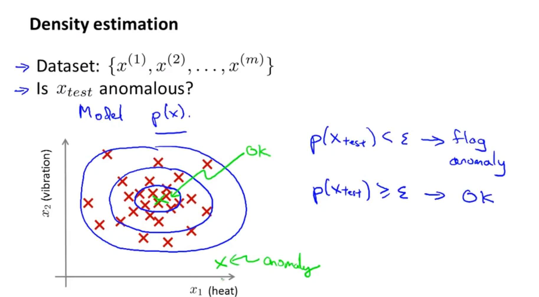
Then, if the probability p of our test set $x_{test}$ is lower than the threshold $\varepsilon$, we label it as anomalous.
The core of anomaly detection is to find a probabilistic model that helps us understand the probability that a sample belongs to the normal samples, thereby helping us distinguish normal samples from anomalous ones. The Gaussian Distribution model is the probability distribution model most commonly used by anomaly detection algorithms.
1. Gaussian Distribution
If x follows a Gaussian distribution, we denote it as: $x\sim N(\mu,\sigma^2)$. Its probability distribution is:
$$p(x;\mu,\sigma^2)=\frac{1}{\sqrt{2\pi}\sigma}exp(-\frac{(x-\mu)^2}{2\sigma^2})$$
where $\mu$ is the expectation (mean), and $\sigma^2$ is the variance.
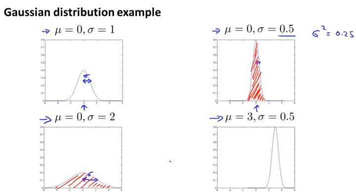
Here, the expectation $\mu$ determines the position of its axis, and the standard deviation $\sigma$ determines how wide or narrow the distribution is. When $\mu=0,\sigma=1$, the normal distribution is the standard normal distribution.
Expectation: $$\mu=\frac{1}{m}\sum_{i=1}^{m}{x^{(i)}}$$
Variance: $$\sigma^2=\frac{1}{m}\sum_{i=1}^{m}{(x^{(i)}-\mu)}^2$$
Suppose we have a set of m unlabeled training examples, and each training example has n features. Then this training set should be a sample matrix composed of m n-dimensional vectors.
In probability theory, parameter estimation over a finite number of samples is:
$$\mu_j = \frac{1}{m} \sum_{i=1}^{m}x_j^{(i)};;;,;;; \delta^2_j = \frac{1}{m} \sum_{i=1}^{m}(x_j^{(i)}-\mu_j)^2$$
The estimates of parameter $\mu$ and parameter $\delta^2$ here are their maximum likelihood estimates.
Assuming that each feature from $x_{1}$ to $x_{n}$ follows a normal distribution, the probability of the model is:
$$
\begin{align*}
p(x)&=p(x_1;\mu_1,\sigma_1^2)p(x_2;\mu_2,\sigma_2^2) \cdots p(x_n;\mu_n,\sigma_n^2)\
&=\prod_{j=1}^{n}p(x_j;\mu_j,\sigma_j^2)\
&=\prod_{j=1}^{n} \frac{1}{\sqrt{2\pi}\sigma_{j}}exp(-\frac{(x_{j}-\mu_{j})^2}{2\sigma_{j}^2})
\end{align*}
$$
When $p(x)<\varepsilon$, $x$ is an anomalous sample.
2. Example
Suppose we have two features, $x_1$ and $x_2$, both of which follow Gaussian distributions. Through parameter estimation, we know the distribution parameters:
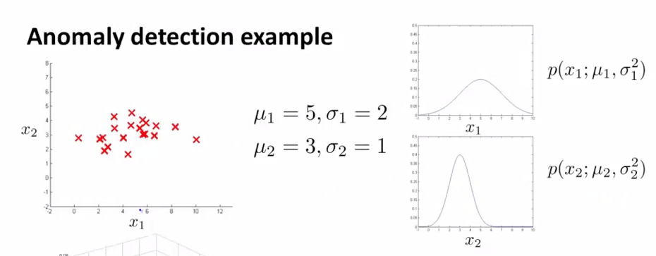
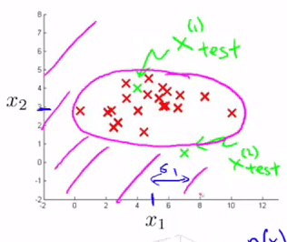
Then the model $p(x)$ can be represented by the following heat map. The hotter the region in the heat map, the higher the probability that a sample is normal. The parameter $\varepsilon$ describes a cutoff height; when the probability falls below the cutoff height (shown as the purple region in the figure below), the sample is anomalous:
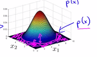
Project $p(x)$ onto the plane containing features $x_1$ and $x_2$. The purple curve in the figure below represents the projection of $\varepsilon$. It is a cutoff curve, and any sample outside this cutoff curve is considered anomalous:
3. Algorithm Evaluation
Because anomalous samples are very rare, the entire dataset is highly skewed. We cannot evaluate an algorithm simply by prediction accuracy. Therefore, we use the Precision and Recall discussed previously to compute the F-score and use it to evaluate anomaly detection algorithms.
- True positive, false positive, true negative, false negative
- Precision and Recall
- F1 Score
We also have a parameter $\varepsilon$. This $\varepsilon$ is the threshold we use to decide when to treat a sample as anomalous. We should try multiple different values of $\varepsilon$ and choose the one that maximizes the F-score.
II. Building an Anomaly Detection System
1. Supervised Learning and Anomaly Detection
| Supervised Learning | Anomaly Detection |
|---|---|
| The data distribution is balanced | The data is highly skewed; the number of anomalous samples is much smaller than the number of normal samples |
| We can learn the form of positive samples by fitting positive samples, and then predict whether a new sample is positive | Anomalies come in many different types, so it is difficult to infer the form of anomalous samples by fitting existing anomalous samples (that is, positive samples) |
The table below shows some application scenarios for the two:
| Supervised Learning | Anomaly Detection |
|---|---|
| Spam detection | Failure detection |
| Weather prediction (predicting rainy, sunny, or cloudy weather) | Monitoring machine equipment in a data center |
| Cancer classification | Determining whether a component is anomalous in manufacturing |
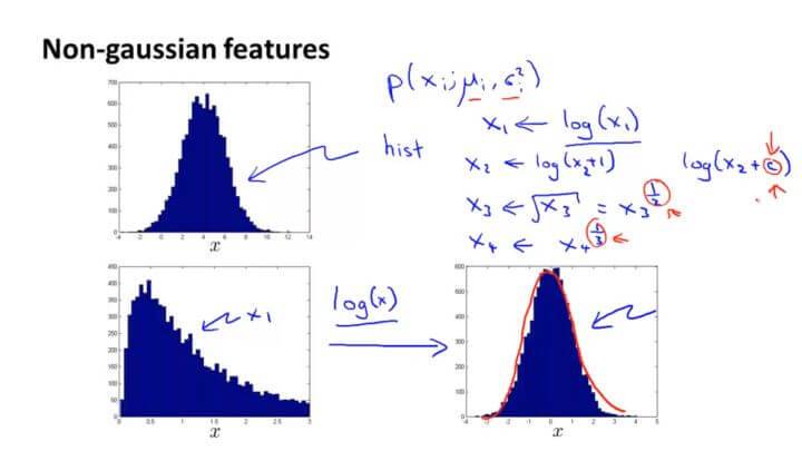
If our data does not appear to follow a Gaussian distribution very well, we can use mathematical transformations such as logarithms, exponentials, and powers to make it closer to a Gaussian distribution.
III. Multivariate Gaussian Distribution (Optional)
1. Multivariate Gaussian Distribution Model
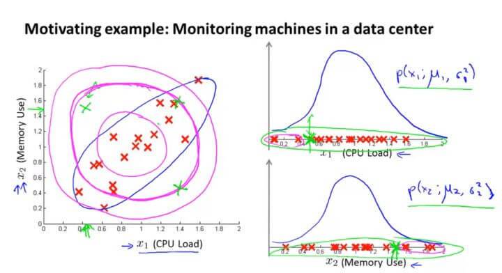
Take monitoring computers in a data center as an example. $x_1$ is the CPU load, and $x_2$ is memory usage. The normal samples are shown as the red points in the left figure. Suppose we have an anomalous sample (the green point in the upper-left corner of the figure). Visually, it is clearly not within the region where the normal samples lie. However, when computing the probability $p(x)$, because it falls within the normal range of the Gaussian distributions for both $x_1$ and $x_2$, this point will not be classified as anomalous.
This is because, in a Gaussian distribution, it cannot perceive that the region with high probability for normal samples is actually the blue ellipse. Its probability decreases gradually outward in circles. Therefore, within the same circle, although the probability is the same in the computation, in practice there is often a large discrepancy.
So we developed an improved version of the anomaly detection algorithm: the multivariate Gaussian distribution.
Instead of computing a Gaussian distribution separately for each feature value, we fit a Gaussian distribution to the entire model.
Its probabilistic model is: $$p(x;\mu,\Sigma)=\frac{1}{(2\pi)^{\frac{n}{2}}|\Sigma|^{\frac{1}{2}}}exp(-\frac{1}{2}(x-\mu)^T\Sigma^{-1}(x-\mu))$$ (where $|\Sigma|$ is the determinant of $\Sigma$, $\mu$ denotes the sample mean, and $\Sigma$ denotes the sample covariance matrix.).
The heat map of the multivariate Gaussian distribution model is as follows:
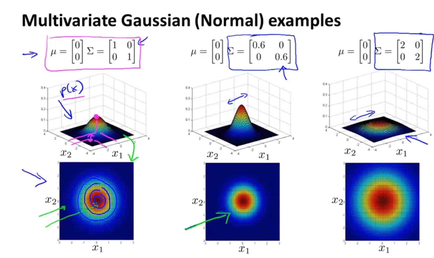
$\Sigma$ is a covariance matrix, so it measures variance. Decreasing $\Sigma$ also decreases its width; increasing it has the opposite effect.
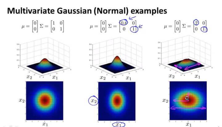
The first number in $\Sigma$ measures $x_1$. If we reduce the first number, we can observe from the figure that the range of $x_1$ is also compressed, turning into an ellipse.
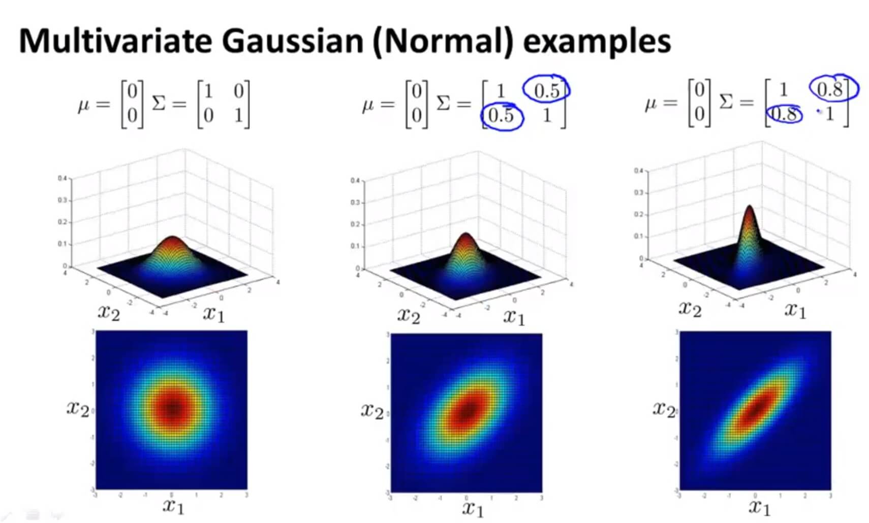
The multivariate Gaussian distribution can also model correlations in the data. If we change the data on the off-diagonal (as shown in the middle figure), then its graph will form a Gaussian distribution along the line $y=x$.
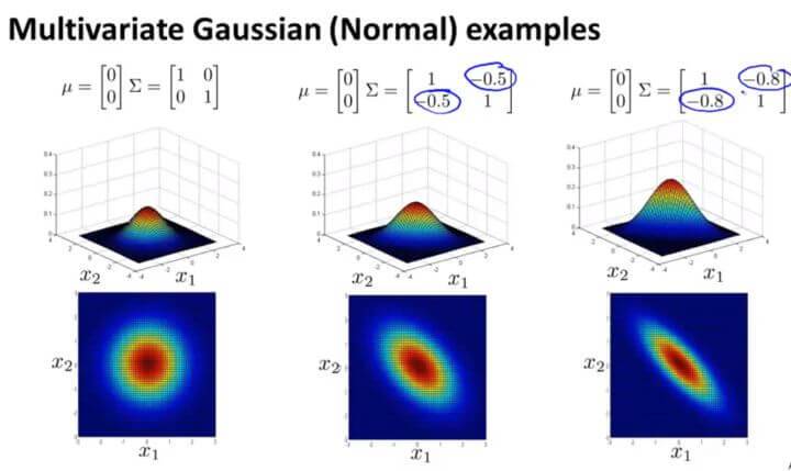
The converse is also true.
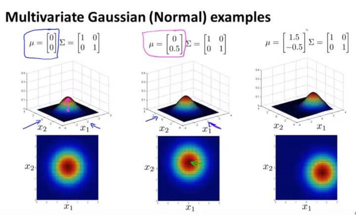
Changing the value of $\mu$ changes the position of its center point.
2. Parameter Estimation
The parameter estimation for the multivariate Gaussian distribution model is as follows:
$$\mu=\frac{1}{m}\sum_{i=1}^{m}{x^{(i)}}$$
$$\Sigma=\frac{1}{m}\sum_{i=1}^{m}{(x^{(i)}-\mu)(x^{(i)}-\mu)^T}$$
3. Algorithm Workflow
The workflow of the anomaly detection algorithm using the multivariate Gaussian distribution is as follows:
- Choose features $x_j$ that are sufficient to reveal anomalous samples.
- Estimate the parameters for each sample: $$\mu=\frac{1}{m}\sum_{i=1}^{m}{x^{(i)}}$$ $$\Sigma=\frac{1}{m}\sum_{i=1}^{m}{(x^{(i)}-\mu)(x^{(i)}-\mu)^T}$$
- When a new sample x arrives, compute $p(x)$: $$p(x)=\frac{1}{(2\pi)^{\frac{n}{2}}|\Sigma|^{\frac{1}{2}}}exp(-\frac{1}{2}(x-\mu)^T\Sigma^{-1}(x-\mu))$$
If $p(x)<\varepsilon $ , then sample x is considered an anomalous sample.
4. Differences Between the Multivariate Gaussian Distribution Model and the General Gaussian Distribution Model
The general Gaussian distribution model is just a constrained version of the multivariate Gaussian distribution model. It constrains the contour lines of the multivariate Gaussian distribution to the axis-aligned distribution shown below (the probability-density contour lines are aligned with the axes):
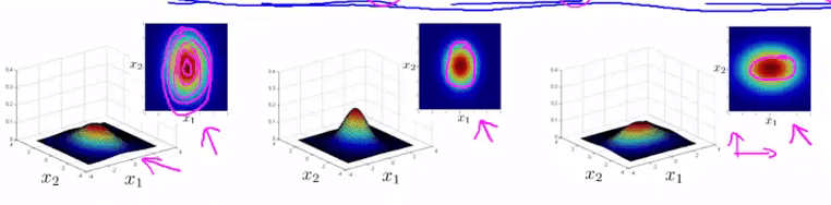
When $\Sigma=\left[ \begin{array}{ccc}\sigma_1^2 \ & \sigma_2^2 \ &&…\&&&\sigma_n^2\end{array} \right]$ , the multivariate Gaussian distribution is the original general Gaussian distribution. (Because there are variances only on the main diagonal, and there are no changes in other slopes.)
Comparison
Model Definition
General Gaussian model:
$$
\begin{align*}
p(x)&=p(x_1;\mu_1,\sigma_1^2)p(x_2;\mu_2,\sigma_2^2) \cdots p(x_n;\mu_n,\sigma_n^2)\
&=\prod_{j=1}^{n}p(x_j;\mu_j,\sigma_j^2)\
&=\prod_{j=1}^{n} \frac{1}{\sqrt{2\pi}\sigma_{j}}exp(-\frac{(x_{j}-\mu_{j})^2}{2\sigma_{j}^2})
\end{align*}
$$
Multivariate Gaussian model:
$$p(x)=\frac{1}{(2\pi)^{\frac{n}{2}}|\Sigma|^{\frac{1}{2}}}exp(-\frac{1}{2}(x-\mu)^T\Sigma^{-1}(x-\mu))$$
Correlation
General Gaussian model:
Some features need to be manually created to describe correlations between certain features.
Multivariate Gaussian model:
Uses the covariance matrix $\Sigma$ to capture correlations among features.
Complexity
General Gaussian model:
Low computational complexity; suitable for high-dimensional features
Multivariate Gaussian model:
Computationally complex
Effectiveness
General Gaussian model:
Works well even when the number of samples m is small
Multivariate Gaussian model:
Requires $\Sigma$ to be invertible, which means $m>n$ is required, and the features must not be linearly correlated. For example, there must not be relationships such as $x_2=3x_1$ or $x_3=x_1+2x_2$
Conclusion: Anomaly detection based on the multivariate Gaussian distribution model has very limited applicability.
IV. Anomaly Detection Test
1. Question 1
For which of the following problems would anomaly detection be a suitable algorithm?
A. Given a dataset of credit card transactions, identify unusual transactions to flag them as possibly fraudulent.
B. Given data from credit card transactions, classify each transaction according to type of purchase (for example: food, transportation, clothing).
C. Given an image of a face, determine whether or not it is the face of a particular famous individual.
D. From a large set of primary care patient records, identify individuals who might have unusual health conditions.
Answer: A, D
Only A and D are suitable for anomaly detection algorithms.
2. Question 2
Suppose you have trained an anomaly detection system for fraud detection, and your system that flags anomalies when $p(x)$ is less than ε, and you find on the cross-validation set that it is missing many fraudulent transactions (i.e., failing to flag them as anomalies). What should you do?
A. Decrease $\varepsilon$
B. Increase $\varepsilon$
Answer: B
3. Question 3
Suppose you are developing an anomaly detection system to catch manufacturing defects in airplane engines. Your model uses
$$p(x) = \prod_{j=1}^{n}p(x_{j};\mu_{j},\sigma_{j}^{2})$$
You have two features $x_1$ = vibration intensity, and $x_2$ = heat generated. Both $x_1$ and $x_2$ take on values between 0 and 1 (and are strictly greater than 0), and for most “normal” engines you expect that $x_1 \approx x_2$. One of the suspected anomalies is that a flawed engine may vibrate very intensely even without generating much heat (large $x_1$, small $x_2$), even though the particular values of $x_1$ and $x_2$ may not fall outside their typical ranges of values. What additional feature $x_3$ should you create to capture these types of anomalies:
A. $x_3 = \frac{x_1}{x_2}$
B. $x_3 = x_1^2\times x_2^2$
C. $x_3 = (x_1 + x_2)^2$
D. $x_3 = x_1 \times x_2^2$
Answer: A
Given features $x_1$ and $x_2$ , you can create feature $x_3=\frac{x_1}{x_2}$ to combine the two.
4. Question 4
Which of the following are true? Check all that apply.
A. When evaluating an anomaly detection algorithm on the cross validation set (containing some positive and some negative examples), classification accuracy is usually a good evaluation metric to use.
B. When developing an anomaly detection system, it is often useful to select an appropriate numerical performance metric to evaluate the effectiveness of the learning algorithm.
C. In a typical anomaly detection setting, we have a large number of anomalous examples, and a relatively small number of normal/non-anomalous examples.
D. In anomaly detection, we fit a model p(x) to a set of negative (y=0) examples, without using any positive examples we may have collected of previously observed anomalies.
Answer: B, D
5. Question 5
You have a 1-D dataset $\begin{Bmatrix} x^{(i)},\cdots,x^{(m)} \end{Bmatrix}$ and you want to detect outliers in the dataset. You first plot the dataset and it looks like this:
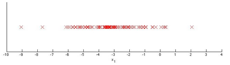
Suppose you fit the gaussian distribution parameters $\mu_1$ and $\sigma_1^2$ to this dataset. Which of the following values for $\mu_1$ and $\sigma_1^2$ might you get?
A. $\mu = -3$,$\sigma_1^2 = 4$
B. $\mu = -6$,$\sigma_1^2 = 4$
C. $\mu = -3$,$\sigma_1^2 = 2$
D. $\mu = -6$,$\sigma_1^2 = 2$
Answer: A
The center point is at -3, and the points around -3, i.e. around (-4, -2), are still relatively dense, so $\sigma_1=2$ .
GitHub Repo: Halfrost-Field
Follow: halfrost · GitHub