Hands-on Neural Network Backpropagation
Because Ghost blogs recognize LaTeX syntax differently from standard LaTeX syntax, and for better generality, the LaTeX formulas in the following article may appear garbled. If that happens and you do not mind, you can read a non-garbled version of this article on the author’s Github. The author will fix this garbling issue when time permits. Thank you for your understanding.
GitHub Repo: Halfrost-Field
Follow: halfrost · GitHub
Source: https://github.com/halfrost/Halfrost-Field/blob/master/contents/Machine_Learning/Backpropagation_in_Practice.ipynb
1. Backpropagation in Practice
To use an optimization algorithm based on gradient descent, we need to use the fminunc function. Its input parameter is $\theta$, and the function returns the cost function jVal and the derivative value gradient. The returned values are then passed to the advanced optimization algorithm fminunc, which outputs the input value @costFunction and the initial value of $\theta$.
Here, the parameters $\Theta_1,\Theta_2,\Theta_3,\cdots$ and $D^{(1)},D^{(2)},D^{(3)},\cdots$ are all matrices. Therefore, in order to call the fminunc function, we need to convert them into vectors.
Suppose we have parameters $\Theta_1,\Theta_2,\Theta_3$ and $D^{(1)},D^{(2)},D^{(3)}$, where Theta1 is $10 * 11$, Theta2 is $10 * 11$, and Theta3 is $1 * 11$.
% Pack into a vector
thetaVector = [ Theta1(:); Theta2(:); Theta3(:); ]
deltaVector = [ D1(:); D2(:); D3(:) ]

% Unpack and restore
Theta1 = reshape(thetaVector(1:110),10,11)
Theta2 = reshape(thetaVector(111:220),10,11)
Theta3 = reshape(thetaVector(221:231),1,11)
So the pattern is:
First expand matrices such as $\Theta_1,\Theta_2,\Theta_3$ into a long vector, assign it to initialTheta, and then pass it into the optimization function fminunc as the initial setting for the theta parameter.
Next, implement the cost function costFunction. The costFunction function takes the parameter thetaVec (the vector that contains all the $\Theta$ parameters from earlier), and then uses the reshape function to recover the initial matrices. This makes it easier to compute the derivatives $D^{(1)},D^{(2)},D^{(3)}$ and the cost function $F(\Theta)$ through forward propagation and backpropagation.
Finally, unroll the results in order to obtain gradientVec, keeping them in the same order as the previously unrolled $\theta$ values. Return these derivative values as a single vector.
II. Gradient Checking
When computing derivatives, we are used to treating them as the derivative at that point. When using gradient descent to compute derivatives, although $F(\Theta)$ may decrease on every iteration, the complexity of backpropagation may still mean that our code contains bugs. One technique called Gradient Checking can reduce the probability of such errors (the causes of this issue are all related to incorrect implementations of backpropagation).
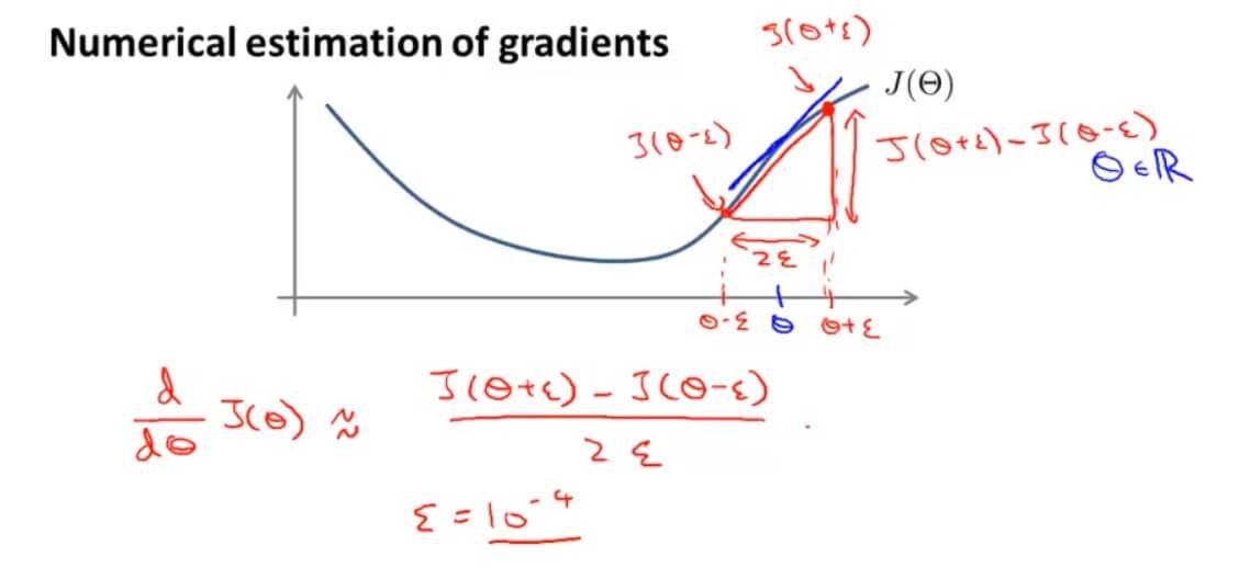
When computing the slope at this point, instead of directly using its derivative, we use $$\frac{d}{d\Theta}F(\Theta)\approx\frac{F(\Theta+\epsilon)-F(\Theta-\epsilon)}{2\epsilon}$$ instead. Usually, $\epsilon$ is chosen to be a small value. (This is essentially using the definition of the derivative.)
The algorithm above is the two-sided difference algorithm. In contrast, the one-sided difference algorithm is:
$$\frac{d}{d\Theta}F(\Theta)\approx\frac{F(\Theta+\epsilon)-F(\Theta)}{\epsilon}$$
Compared with the one-sided difference, the two-sided difference can produce more accurate results.
Generalizing the two-sided difference:
$$\frac{d}{d\Theta_j}J(\Theta)\approx\frac{J(\Theta_1,…,+\Theta_j+\epsilon,…,\Theta_n)-J(\Theta_1,…,+\Theta_j-\epsilon,…,\Theta_n)}{2\epsilon}$$
The corresponding code implementation is as follows:
epsilon = 1e-4;
for i = 1:n,
  thetaPlus = theta;
  thetaPlus(i) += epsilon;
  thetaMinus = theta;
  thetaMinus(i) -= epsilon;
  gradApprox(i) = (J(thetaPlus) - J(thetaMinus))/(2*epsilon)
end;
Compare the derivative DVec computed by backpropagation with gradApprox computed by the program above. If $gradApprox \approx DVec$, it indicates that the backpropagation implementation is correct.
Finally, disable gradient checking when using the algorithm for learning. Gradient checking is mainly intended to help us determine whether there are bugs in the algorithm implementation we wrote; it is not meant to compute derivatives, because this method is much slower than the previous approach for computing derivatives.
To summarize:
- Compute DVec using backpropagation; DVec is the packed and unrolled form of each matrix.
- Implement numerical gradient checking to compute gradApprox.
- Compare whether $gradApprox \approx DVec$ is equal or approximately equal.
- Remember to disable gradient checking when using the algorithm for learning. Gradient checking should only be performed during the code testing phase.
III. Random Initialization
When using the gradient descent algorithm, you need to set the initial value of $\Theta$.
optTheta = fminunc(@costFunction, initialTheta, options)
When calling the fminunc function, if initialTheta is initialized entirely to 0,
initialTheta = zeros(n,1)
In the earlier linear regression and logistic regression cases, using gradient functions with the initial values set to 0 is fine. However, in neural networks, doing the same will lead to a high degree of redundancy.
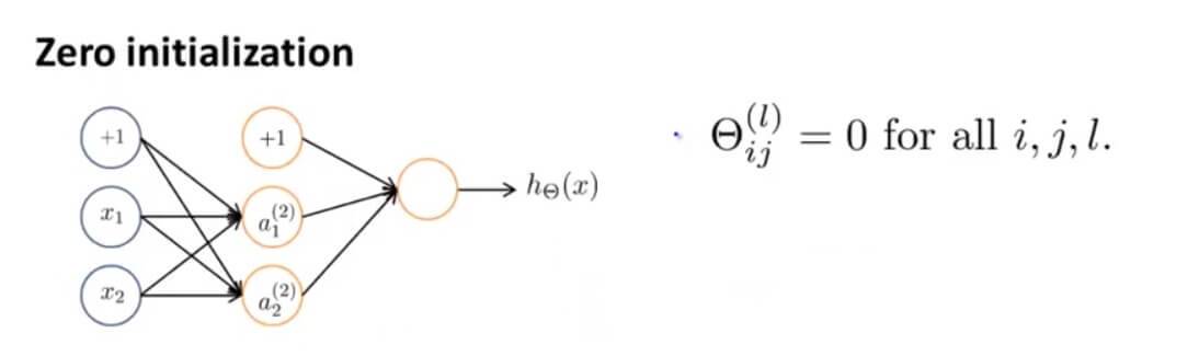
Suppose we have such a network, and all of its initial parameters are set to 0. We will find that its activations satisfy $a_1^{(2)}=a_2^{(2)}$, the errors satisfy $\delta_1^{(2)}=\delta_2^{(2)}$, and the derivatives satisfy $\frac{d}{d\Theta^{(1)}{01}}J(\Theta)=\frac{d}{d\Theta^{(1)}{02}}J(\Theta)$. As a result, when the parameters are updated, the two parameters remain the same. No matter how many times the computation is repeated, the activations on both sides are still identical.
The issue above is called the symmetric weights problem, where all weights are the same. Random initialization is the way to solve this problem.
We restrict the initialization range of the weights $\Theta_{ij}^{(l)}$ to $[-\Phi ,\Phi ]$.
The code representation is as follows:
%If the dimensions of Theta1 is 10x11, Theta2 is 10x11 and Theta3 is 1x11.

Theta1 = rand(10,11) * (2 * INIT_EPSILON) - INIT_EPSILON;
Theta2 = rand(10,11) * (2 * INIT_EPSILON) - INIT_EPSILON;
Theta3 = rand(1,11) * (2 * INIT_EPSILON) - INIT_EPSILON;
rand(x,y) is a random function that initializes a matrix of random real numbers between 0 and 1.
IV. Summary
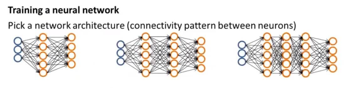
1. Preparation
First, we need to determine how many input units the neural network has, how many hidden layers it has, how many units each hidden layer contains, and how many output units it has. How should we choose these values?
- The number of input units is the dimension of the feature vector $x^{(i)}$
- The number of output units is the number of classes
- In general, the more units in each hidden layer, the better (this must be balanced against computational cost, which increases as more hidden units are added)
- Default: 1 hidden layer. If there are multiple hidden layers, it is recommended that each hidden layer have the same number of units.
If this is a multiclass classification problem, the output units need to be represented in matrix form:
For example, if there are 3 classes, the output units should be written as
$$ \begin{align*} y = \begin{bmatrix} 1\ 0\ 0 \ \end{bmatrix} or \begin{bmatrix} 0\ 1\ 0 \ \end{bmatrix} or \begin{bmatrix} 0\ 0\ 1\ \end{bmatrix} \end{align*} $$
2. Training
Step 1: Randomly initialize the weights. The initialized values are random, small, and close to zero.
Step 2: Run the forward propagation algorithm and compute the hypothesis function $h_\Theta(x^{(i)})$ for each $x^{(i)}$.
Step 3: Compute the cost function $F(\Theta)$.
Step 4: Run the backpropagation algorithm and compute the partial derivative $\frac{\partial}{\partial\Theta_{jk}^{(l)}}F(\Theta)$.
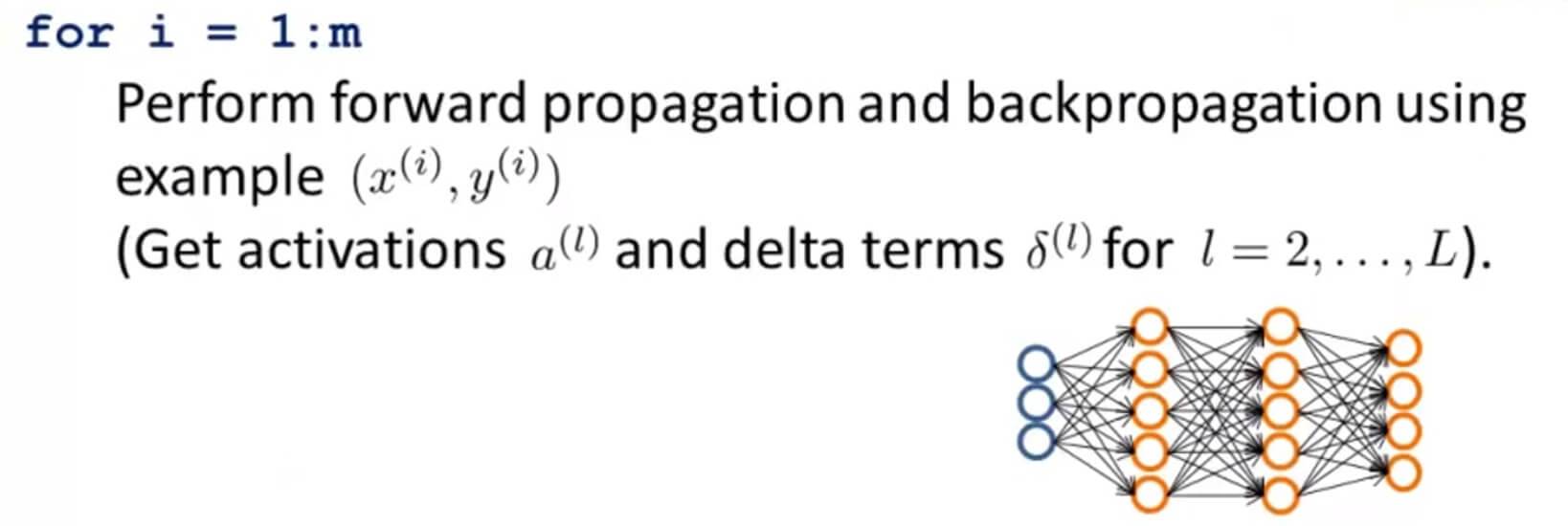
In practice, this means using a for loop: first perform one forward propagation and backpropagation pass on $(x^{(1)},y^{(1)})$, then perform the same operations on $(x^{(2)},y^{(2)})$, continuing all the way through $(x^{(n)},y^{(n)})$. This gives us the activation value corresponding to each unit in each layer of the neural network, as well as the error $\delta^{(l)}$ for each layer’s activations.
Step 5: Use gradient checking to compare whether the partial derivative terms computed by backpropagation are approximately equal to the derivative terms computed by the gradient checking algorithm. Remember to delete this gradient checking code after the check is complete.
Step 6: Finally, use gradient descent or a more advanced algorithm such as LBFGS or conjugate gradient, together with the previously computed partial derivative terms, to minimize the cost function $F(\Theta)$ and compute the weights $\Theta$.
Ideally, as long as $h_{\Theta}(x^{(i)})\approx y^{(i)}$ is satisfied, we can minimize the cost function. However, the cost function $F(\Theta)$ is not convex, so in the end we may use a local minimum as a substitute for the global minimum.
V. Neural Networks: Learning Quiz
1. Question 1
You are training a three layer neural network and would like to use backpropagation to compute the gradient of the cost function. In the backpropagation algorithm, one of the steps is to update
$\Delta^{(2)}{ij}:=\Delta^{(2)}{ij}+\delta^{(3)}{i}*(a^{(2)}){j}$
for every i,j. Which of the following is a correct vectorization of this step?
A. $\Delta^{(2)}:=\Delta^{(2)}+(a^{(3)})^T * \delta^{(2)} $
B. $\Delta^{(2)}:=\Delta^{(2)}+(a^{(2)})^T * \delta^{(3)} $
C. $\Delta^{(2)}:=\Delta^{(2)}+\delta^{(3)}(a^{(3)})^T $
D. $\Delta^{(2)}:=\Delta^{(2)}+\delta^{(3)}(a^{(2)})^T $
Answer: D
2. Question 2
Suppose Theta1 is a 5x3 matrix, and Theta2 is a 4x6 matrix. You set thetaVec=[Theta1(:);Theta2(:)]. Which of the following correctly recovers Theta2?
A. reshape(thetaVec(16:39),4,6)
B. reshape(thetaVec(15:38),4,6)
C. reshape(thetaVec(16:24),4,6)
D. reshape(thetaVec(15:39),4,6)
E. reshape(thetaVec(16:39),6,4)
Answer: A
3. Question 3
Let $J(\theta)=2\theta^3+2$ . Let $\theta=1$ , and $\epsilon=0.01$ . Use the formula $\frac{J(\theta+\epsilon)-J(\theta-\epsilon)}{2\epsilon}$ to numerically compute an approximation to the derivative at $\theta=1$ . What value do you get? (When $\theta=1$ , the true/exact derivati ve is $\frac{dJ(\theta)}{d\theta}=6$ .)
A.6
B.8
C.5.9998
D.6.0002
Answer: D
4. Question 4
Which of the following statements are true? Check all that apply.
A. Gradient checking is useful if we are using gradient descent as our optimization algorithm. However, it serves little purpose if we are using one of the advanced optimization methods (such as in fminunc).
B. If our neural network overfits the training set, one reasonable step to take is to increase the regularization parameter λ .
C. Using gradient checking can help verify if one’s implementation of backpropagation is bug-free.
D. Using a large value of λ cannot hurt the performance of your neural network; the only reason we do not set λ to be too large is to avoid numerical problems.
E. For computational efficiency, after we have performed gradient checking to verify that our backpropagation code is correct, we usually disable gradient checking before using backpropagation to train the network.
F. Computing the gradient of the cost function in a neural network has the same efficiency when we use backpropagation or when we numerically compute it using the method of gradient checking.
Answer: B, C, E
A. Gradient checking is only used to verify whether the algorithm we use to compute partial derivatives is correct; it is not used for computation during training.
B. Increasing the regularization parameter λ to address overfitting is correct.
C. Gradient checking can verify whether the backpropagation algorithm is correct.
D. If the regularization parameter λ is too large, it will cause underfitting.
E. This is again saying that gradient checking can verify the correctness of the backpropagation algorithm.
F. This is again saying that gradient checking can be used to compute partial derivatives inside the algorithm.
5. Question 5
Which of the following statements are true? Check all that apply.
A. Suppose you have a three layer network with parameters $\Theta^{(1)}$ (controlling the function mapping from the inputs to the hidden units) and $\Theta^{(2)}$ (controlling the mapping from the hidden units to the outputs). If we set all the elements of $\Theta^{(1)}$ to be 0, and all the elements of $\Theta^{(2)}$ to be 1, then this suffices for symmetry breaking, since the neurons are no longer all computing the same function of the input.
B. If we are training a neural network using gradient descent, one reasonable “debugging” step to make sure it is working is to plot $J(\Theta)$ as a function of the number of iterations, and make sure it is decreasing (or at least non-increasing) after each iteration.
C. Suppose you are training a neural network using gradient descent. Depending on your random initialization, your algorithm may converge to different local optima (i.e., if you run the algorithm twice with different random initializations, gradient descent may converge to two different solutions). D. If we initialize all the parameters of a neural network to ones instead of zeros, this will suffice for the purpose of “symmetry breaking” because the parameters are no longer symmetrically equal to zero.
E. If we are training a neural network using gradient descent, one reasonable “debugging” step to make sure it is working is to plot $J(\Theta)$ as a function of the number of iterations, and make sure it is decreasing (or at least non-increasing) after each iteration.
F. Suppose we have a correct implementation of backpropagation, and are training a neural network using gradient descent. Suppose we plot $J(\Theta)$ as a function of the number of iterations, and find that it is increasing rather than decreasing. One possible cause of this is that the learning rate $\alpha$ is too large.
G. Suppose that the parameter $\Theta^{(1)}$ is a square matrix (meaning the number of rows equals the number of columns). If we replace $\Theta^{(1)}$ with its transpose $(\Theta^{(1)})^T$ , then we have not changed the function that the network is computing.
H. Suppose we are using gradient descent with learning rate $\alpha$ . For logistic regression and linear regression, $J(\Theta)$ was a convex optimization problem and thus we did not want to choose a learning rate $\alpha$ that is too large. For a neural network however, $J(\Theta)$ may not be convex, and thus choosing a very large value of $\alpha$ can only speed up convergence.
Answer: B, C, F
A. If all the weights in a layer are the same number, symmetry cannot be broken.
B. It is correct that as the number of iterations increases, the cost function $J(\Theta)$ decreases.
C. It is correct that if the learning rate $\alpha$ is too large, the cost function may increase as the number of iterations increases.
D. Setting all weights to 1 also cannot break symmetry.
E. Ensuring that $J(\Theta)$ decreases as the number of iterations increases can be used to verify that the algorithm is correct.
F. Same as B.
G. The transpose of a matrix is generally not equal to the original matrix.
H. Choosing a large learning rate $\alpha$ can cause $J(\Theta)$ to fail to converge.
GitHub Repo: Halfrost-Field
Follow: halfrost · GitHub