PCA and Dimensionality Reduction
Because Ghost Blog recognizes LaTeX syntax differently from standard LaTeX syntax, some LaTeX formulas in the following article may appear garbled for better generality. If that happens, and if you do not mind, you can read the ungarbled version of this article on the author’s Github. The author will fix this garbling issue when time permits. Thank you for your understanding.
GitHub Repo: Halfrost-Field
Follow: halfrost · GitHub
Source: https://github.com/halfrost/Halfrost-Field/blob/master/contents/Machine_Learning/Dimensionality_Reduction.ipynb
I. Motivation
We would very much like to have sufficiently many features (knowledge) to ensure the training effectiveness of a learning model. Especially in tasks such as image processing, high-dimensional features are unavoidable. However, high-dimensional features also have several drawbacks:
- Learning performance decreases. The more knowledge there is, the slower it becomes to absorb the knowledge (input) and master it (learning).
- Too many features are hard to distinguish. It is difficult to immediately understand what a particular feature represents.
- Feature redundancy. As shown in the figure below, centimeters and feet are a pair of redundant features: they represent the same meaning and can be converted into each other.
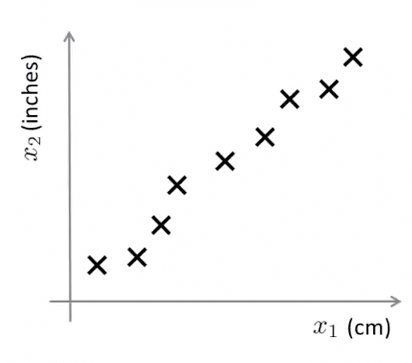
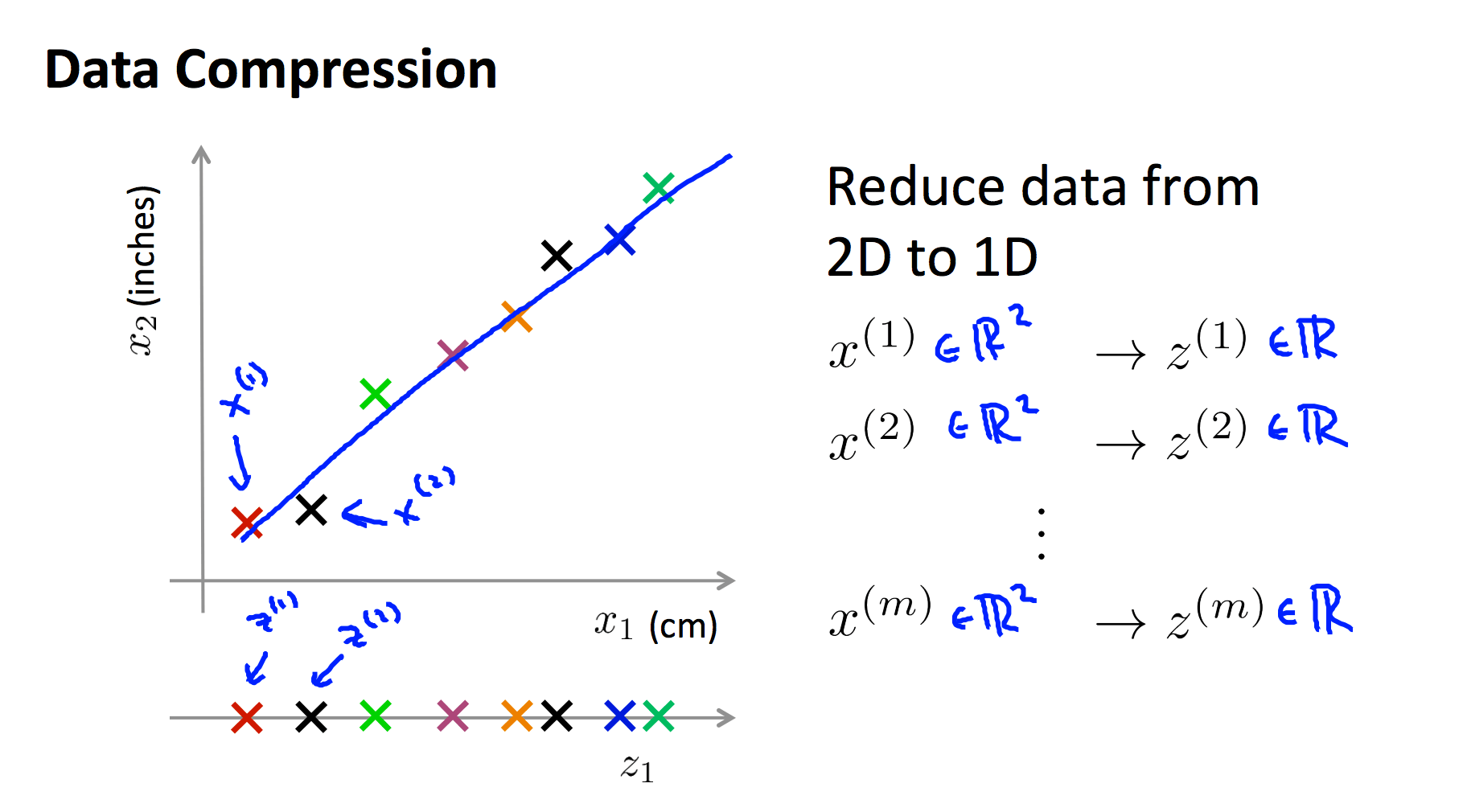
Here we use a green straight line and project each sample onto that line. The original two-dimensional feature x=(centimeters, feet) is thus reduced to a one-dimensional feature x=(relative position on the line).
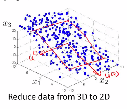
In the example below, we project three-dimensional features onto a two-dimensional plane, thereby reducing the three-dimensional features to two dimensions:
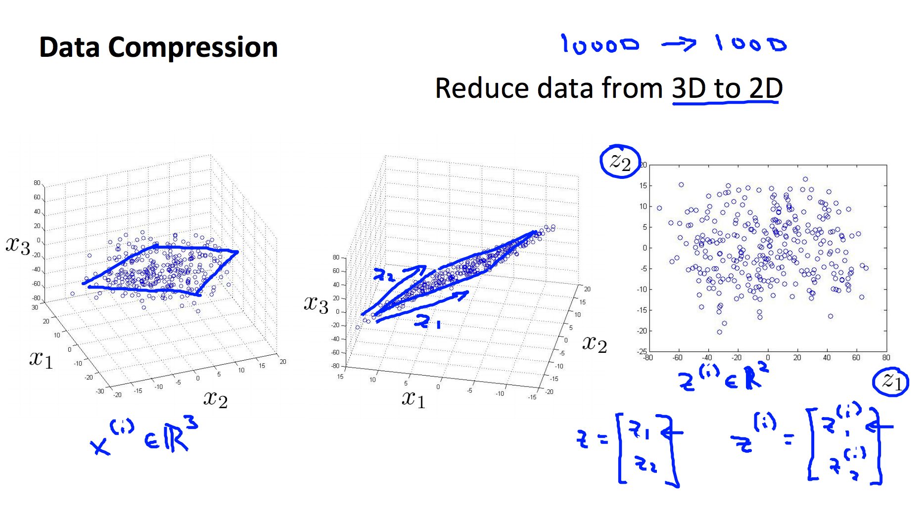
The general approach to feature dimensionality reduction is to project high-dimensional features into a low-dimensional space.
II. Principal Component Analysis
PCA, Principal Component Analysis, is the most commonly used method for feature dimensionality reduction. As the name suggests, PCA can extract the principal components from redundant features and improve model training speed without significantly degrading model quality.
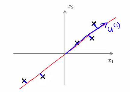
As shown in the figure above, we call the distance from a sample to the red vector the projection error. Taking the projection from two dimensions to one dimension as an example, PCA seeks a straight line such that the projection error of each feature is sufficiently small, so that as much information from the original features as possible is retained.
Suppose we want to reduce the features from n dimensions to k dimensions. PCA first finds k n-dimensional vectors, then projects the features into the k-dimensional space formed by these vectors, while ensuring that the projection error is sufficiently small. In the figure below, in order to reduce the feature dimension from three dimensions to two, PCA first finds two three-dimensional vectors $\mu^{(1)},\mu^{(2)}$; together they form a two-dimensional plane, and the original three-dimensional features are then projected onto that two-dimensional plane:
1. Differences
The difference between PCA and linear regression is:
Linear regression looks for the minimum distance perpendicular to the X-axis, while PCA looks for the minimum perpendicular projection distance.
2. Algorithm Workflow
Assume we need to reduce the feature dimension from n dimensions to k dimensions. The PCA procedure is as follows:
Standardize the features to balance the scale of each feature:
$$x^{(i)}_j=\frac{x^{(i)}_j-\mu_j}{s_j}$$
$\mu_j$ is the mean of feature j, and sj is the standard deviation of feature j.
Compute the covariance matrix $\Sigma $:
$$\Sigma =\frac{1}{m}\sum_{i=1}{m}(x^{(i)})(x^{(i)})^T=\frac{1}{m} \cdot X^TX$$
Use singular value decomposition (SVD) to compute the eigenvectors of $\Sigma $:
$$(U,S,V^T)=SVD(\Sigma )$$
Take the first k left singular vectors from U to form a reduced matrix Ureduce:
$$U_{reduce}=(\mu^{(1)},\mu^{(2)},\cdots,\mu^{(k)})$$
Compute the new feature vector: $z^{(i)}$
$$z^{(i)}=U^{T}_{reduce} \cdot x^{(i)}$$
3. Feature Reconstruction
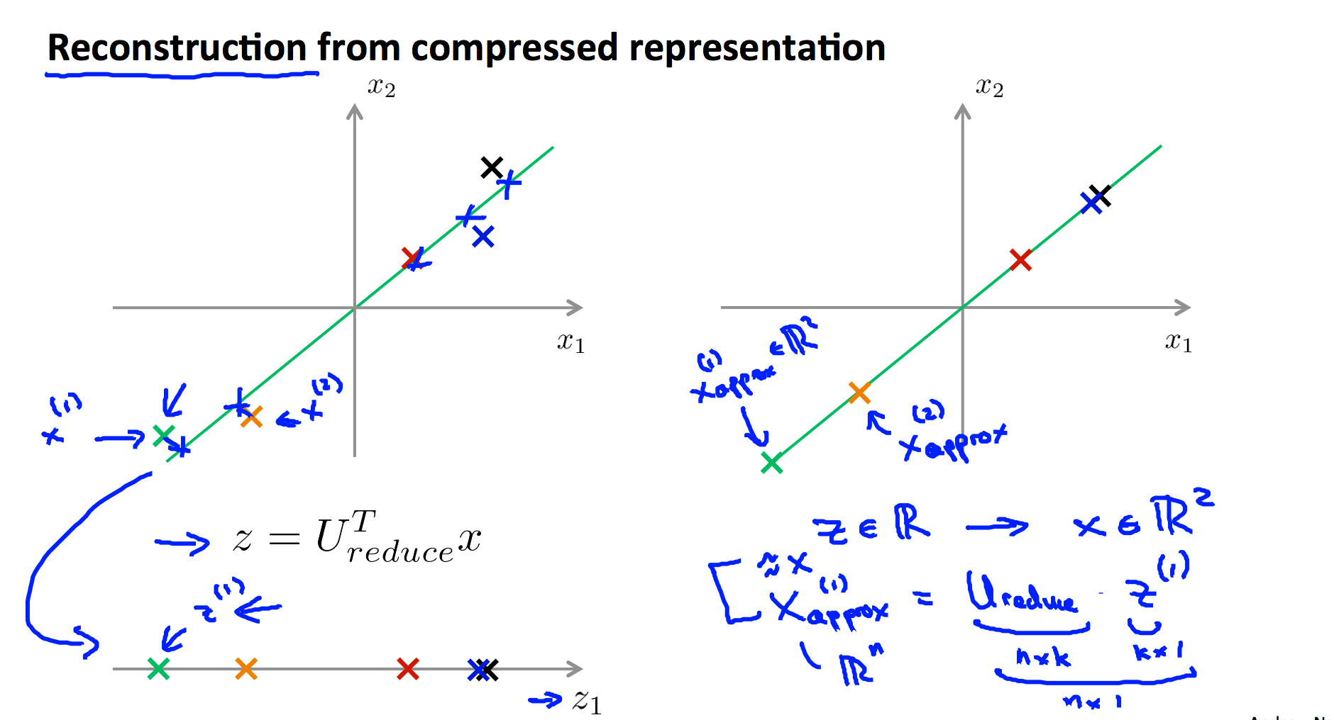
Because PCA retains only the principal components of the features, it is a lossy compression method. Suppose the new feature vector we obtain is:
$$z=U^T_{reduce}x$$
Then the reconstructed feature $x_{approx}$ is:
$$x_{approx}=U_{reduce}z$$
4. How Much Dimensionality Reduction Is Appropriate?
From the PCA procedure, we know that we need to specify the target dimension k for PCA. If the dimensionality reduction is too small, the performance improvement will be limited; if the target dimension is too small, too much information will be lost. Typically, the following procedure is used to evaluate whether the choice of k is good:
Compute the mean squared projection error for all samples:
$$\min \frac{1}{m}\sum_{j=1}^{m}\left | x^{(i)}-x^{(i)}_{approx} \right |^2$$
Compute the total variation of the data:
$$\frac{1}{m}\sum_{j=1}^{m}\left | x^{(i)} \right |^2$$
Evaluate whether the following inequality holds:
$$\frac{\min \frac{1}{m}\sum_{j=1}^{m}\left | x^{(i)}-x^{(i)}_{approx} \right |^2}{\frac{1}{m}\sum_{j=1}^{m}\left | x^{(i)} \right |^2} \leqslant \epsilon $$
Here, $\epsilon $ can take values such as 0.01,0.05,0.10,⋯0.01,0.05,0.10,⋯. Suppose $\epsilon = 0.01 $; then we say that “99% of the variance among the features is retained.”
5. Do Not Optimize Prematurely
Because PCA reduces the feature dimension, it may also introduce overfitting issues. PCA is not mandatory. In machine learning, always remember not to optimize prematurely. Only when the algorithm’s runtime efficiency is unsatisfactory should you consider using PCA or other feature dimensionality reduction techniques to improve training speed.
When you retain 99%, 95%, or some other percentage of the variance, the results indicate that simply using regularization will give you a very good way to avoid overfitting. Regularization often works better than PCA, because when you use linear regression, logistic regression, or other methods together with regularization, the minimization problem is still informed by the y values, which helps avoid discarding useful information. PCA, however, does not use these labels, so it is more likely to discard valuable information. In short, using PCA to speed up a learning algorithm is a good application, but using it to avoid overfitting is not a good application of PCA. Replacing PCA with regularization is what many people recommend.
If your learning algorithm converges very slowly, or consumes a very large amount of memory or disk space, you may want to compress the data. Only when your $x^{(i)}$ performs poorly—only when you have evidence or sufficient reason to determine that $x^{(i)}$ is not working well—should you consider using PCA to compress the data.
PCA is typically used to compress data, reduce memory usage or disk space usage, or visualize data.
III. Principal Component Analysis Test
1. Question 1
Consider the following 2D dataset:
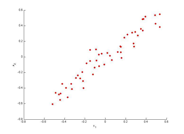
Which of the following figures correspond to possible values that PCA may return for u(1) (the first eigenvector / first principal component)? Check all that apply (you may have to check more than one figure).
A. 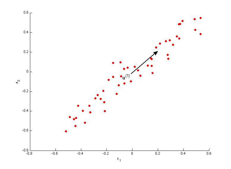
B. 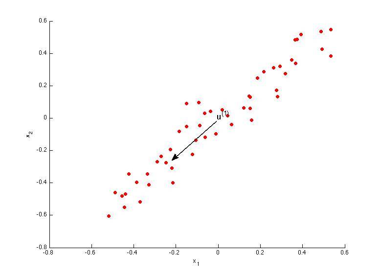
C. 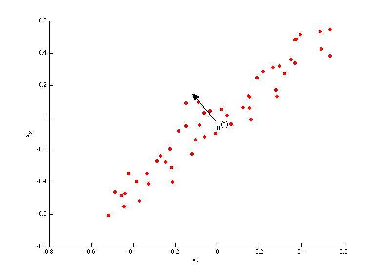
D. 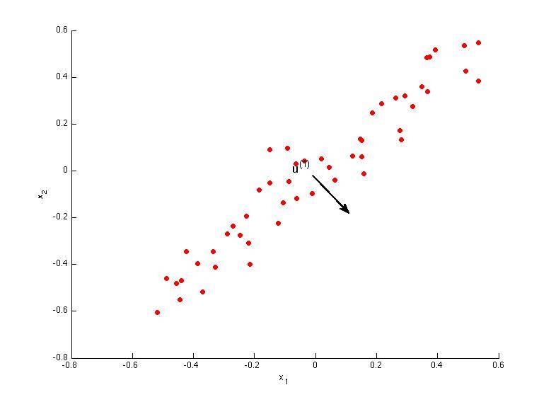
Answer: A, B
2. Question 2
Which of the following is a reasonable way to select the number of principal components k?
(Recall that n is the dimensionality of the input data and m is the number of input examples.)
A. Choose k to be the smallest value so that at least 1% of the variance is retained.
B. Choose k to be the smallest value so that at least 99% of the variance is retained.
C. Choose the value of k that minimizes the approximation error $\frac{1}{m}\sum^{m}{i=1}\left | x^{(i)} - x{approx}^{(i)} \right |^{2}$.
D. Choose k to be 99% of n (i.e., k=0.99∗n, rounded to the nearest integer). Answer: B
3. Question 3
Suppose someone tells you that they ran PCA in such a way that “95% of the variance was retained.” What is an equivalent statement to this?
A. $\frac{\frac{1}{m}\sum^{m}{i=1}\left | x^{(i)} \right |^{2}}{\frac{1}{m}\sum^{m}{i=1}\left | x^{(i)} - x_{approx}^{(i)} \right |^{2}} \geqslant 0.05$
B. $\frac{\frac{1}{m}\sum^{m}{i=1}\left | x^{(i)} \right |^{2}}{\frac{1}{m}\sum^{m}{i=1}\left | x^{(i)} - x_{approx}^{(i)} \right |^{2}} \leqslant 0.95$
C. $\frac{\frac{1}{m}\sum^{m}{i=1}\left | x^{(i)} - x{approx}^{(i)} \right |^{2}}{\frac{1}{m}\sum^{m}_{i=1}\left | x^{(i)} \right |^{2}} \leqslant 0.05$
D. $\frac{\frac{1}{m}\sum^{m}{i=1}\left | x^{(i)} \right |^{2}}{\frac{1}{m}\sum^{m}{i=1}\left | x^{(i)} - x_{approx}^{(i)} \right |^{2}} \leqslant 0.05$
Answer: C
4. Question 4
Which of the following statements are true? Check all that apply.
A. If the input features are on very different scales, it is a good idea to perform feature scaling before applying PCA.
B. Feature scaling is not useful for PCA, since the eigenvector calculation (such as using Octave’s svd(Sigma) routine) takes care of this automatically.
C. Given an input $x \in \mathbb{R}^{n}$, PCA compresses it to a lower-dimensional vector $z \in \mathbb{R}^{k}$.
D. PCA can be used only to reduce the dimensionality of data by 1 (such as 3D to 2D, or 2D to 1D).
Answer: A, C
5. Question 5
Which of the following are recommended applications of PCA? Select all that apply.
A. To get more features to feed into a learning algorithm.
B. Data compression: Reduce the dimension of your data, so that it takes up less memory / disk space.
C. Data visualization: Reduce data to 2D (or 3D) so that it can be plotted.
D. Data compression: Reduce the dimension of your input data $x^{(i)}$, which will be used in a supervised learning algorithm (i.e., use PCA so that your supervised learning algorithm runs faster).
Answer: B, C
GitHub Repo: Halfrost-Field
Follow: halfrost · GitHub