How to Design and Implement a Thread-Safe Map? (Part 1)
Map is a very common data structure used to store unordered key-value pairs. Most mainstream programming languages provide a built-in implementation by default. C and C++ have Map implementations in the STL, JavaScript has Map, Java has HashMap, Swift and Python have Dictionary, Go has Map, and Objective-C has NSDictionary and NSMutableDictionary.
Are all of these Maps thread-safe? The answer is no—not all of them are thread-safe. So how can we implement a thread-safe Map? To answer that question, we first need to start with how to implement a Map.
I. What Data Structure Should Be Used to Implement a Map?
Map is a very commonly used data structure: a collection of unordered key/value pairs, where all keys in a Map are distinct. Given a key, the corresponding value can be looked up, updated, or deleted in constant time, O(1).
To achieve constant-time lookup, what should we use for the implementation? Readers will probably think of a hash table right away. Indeed, the underlying implementation of a Map is generally an array, with the help of a hashing algorithm. For a given key, a hash operation is usually performed first, and then the result is taken modulo the length of the hash table to map the key to a specific location.
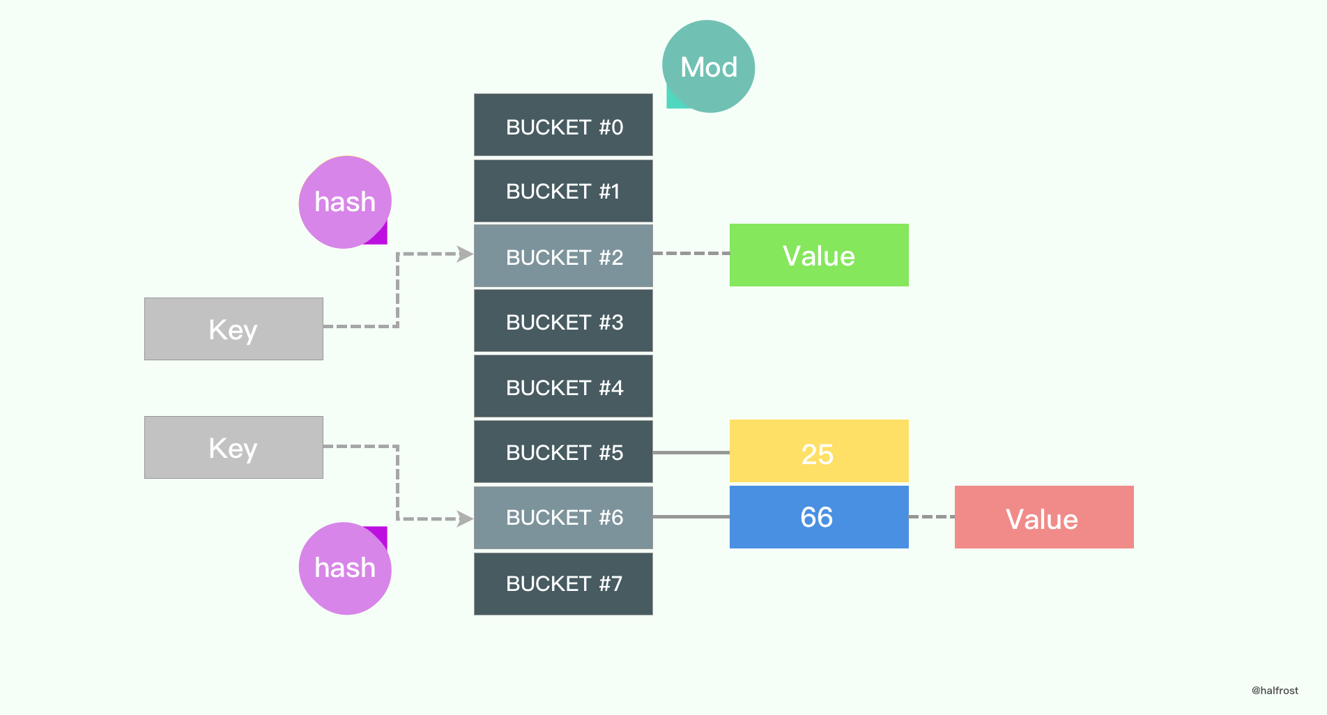
There are many kinds of hashing algorithms. Which one is more efficient?
1. Hash Functions
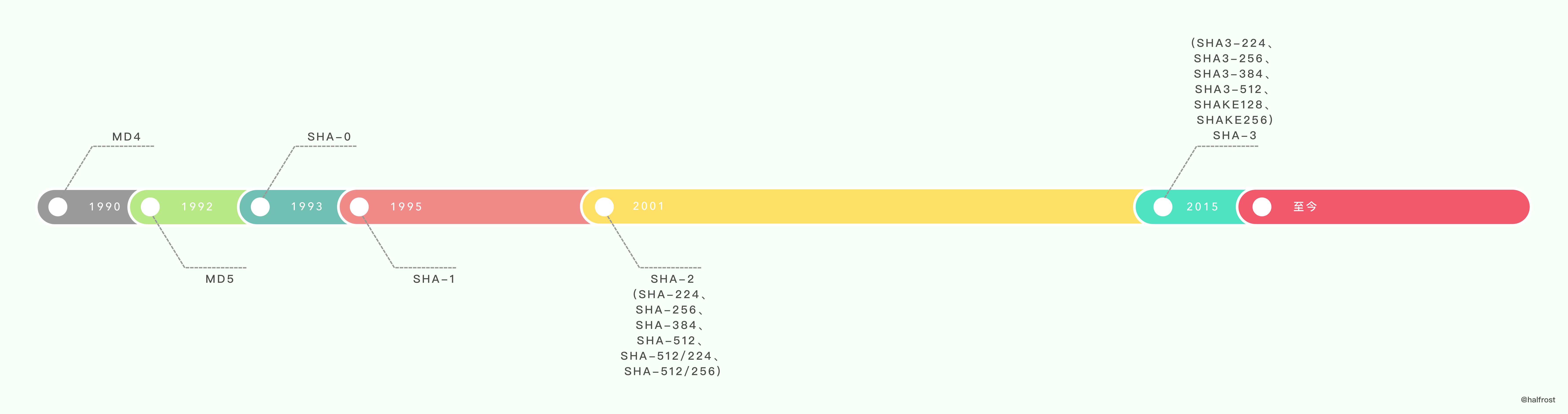
MD5 and SHA1 are arguably the most widely used hash algorithms today, and both were designed based on MD4.
MD4 (RFC 1320) was designed by MIT’s Ronald L. Rivest in 1990. MD stands for Message Digest. It is suitable for high-speed software implementations on processors with a 32-bit word size—it is implemented using bit operations on 32-bit operands. MD5 (RFC 1321) is Rivest’s improved version of MD4 from 1991. It still processes input in 512-bit blocks, and its output is the concatenation of four 32-bit words, the same as MD4. MD5 is more complex than MD4 and slightly slower, but it is more secure and performs better against cryptanalysis and differential attacks.
SHA1 was designed by NIST and the NSA for use with DSA. For inputs with length less than 264, it produces a 160-bit hash value, so it has better resistance to brute-force attacks. SHA-1 was designed based on the same principles as MD4 and imitates that algorithm.
Common hash functions include SHA-1, SHA-256, SHA-512, and MD5. These are classic hash algorithms. In modern production systems, more modern hash algorithms are also used. Below, we list a few of them, compare their performance, and finally choose one implementation to analyze its source code.
(1) Jenkins Hash and SpookyHash
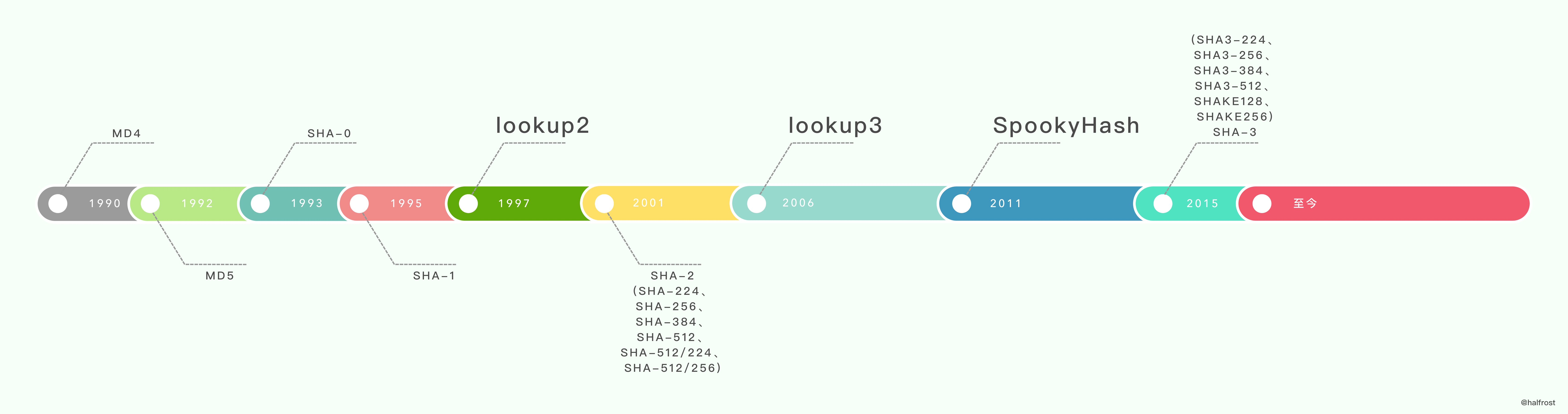
In 1997, Bob Jenkins published an article on hash functions in Dr. Dobbs Journal, titled “A hash function for hash Table lookup”. In that article, Bob covered a broad range of existing hash functions, including one he called “lookup2.” Later, in 2006, Bob released lookup3. lookup3 is Jenkins Hash. For more information about Bob’s hash functions, see Wikipedia: Jenkins hash function. memcached’s hash algorithm supports two algorithms: jenkins and murmur3; the default is jenkins.
In 2011, Bob Jenkins released a new hash function of his own: SpookyHash (so named because it was released on Halloween). Both are twice as fast as MurmurHash, but they use only 64-bit mathematical functions and have no 32-bit version. SpookyHash produces a 128-bit output.
(2) MurmurHash
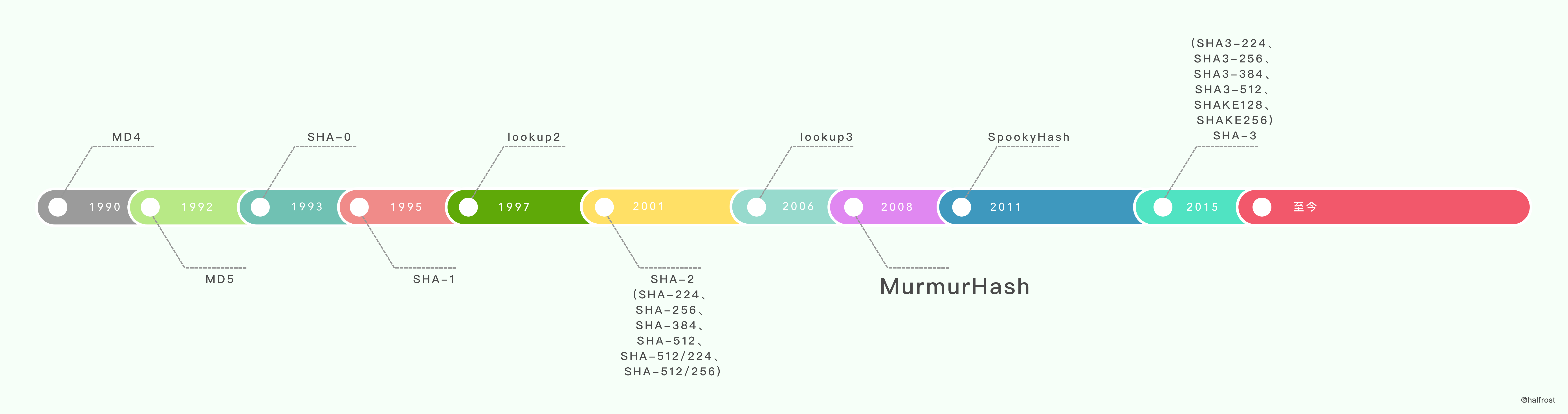
MurmurHash is a non-cryptographic hash function, suitable for general hash-based lookup operations.
In 2008, Austin Appleby released a new hash function—MurmurHash. Its latest version is roughly twice as fast as lookup3 (about 1 byte/cycle), and it has both 32-bit and 64-bit versions. The 32-bit version uses only 32-bit mathematical functions and produces a 32-bit hash value, while the 64-bit version uses 64-bit mathematical functions and produces a 64-bit hash value. According to Austin’s analysis, MurmurHash has excellent performance, although Bob Jenkins claimed in Dr. Dobbs article: “I predict MurmurHash is weaker than lookup3, but I don’t know by how much, because I haven’t tested it yet.” MurmurHash became popular quickly thanks to its excellent speed and statistical properties. The current version is MurmurHash3, and Redis, Memcached, Cassandra, HBase, and Lucene all use it.
Below is a MurmurHash implementation in C:
uint32_t murmur3_32(const char *key, uint32_t len, uint32_t seed) {
        static const uint32_t c1 = 0xcc9e2d51;
        static const uint32_t c2 = 0x1b873593;
        static const uint32_t r1 = 15;
        static const uint32_t r2 = 13;
        static const uint32_t m = 5;
        static const uint32_t n = 0xe6546b64;

        uint32_t hash = seed;

        const int nblocks = len / 4;
        const uint32_t *blocks = (const uint32_t *) key;
        int i;
        for (i = 0; i < nblocks; i++) {
                uint32_t k = blocks[i];
                k *= c1;
                k = (k << r1) | (k >> (32 - r1));
                k *= c2;

                hash ^= k;
                hash = ((hash << r2) | (hash >> (32 - r2))) * m + n;
        }

        const uint8_t *tail = (const uint8_t *) (key + nblocks * 4);
        uint32_t k1 = 0;

        switch (len & 3) {
        case 3:
                k1 ^= tail[2] << 16;
        case 2:
                k1 ^= tail[1] << 8;
        case 1:
                k1 ^= tail[0];

                k1 *= c1;
                k1 = (k1 << r1) | (k1 >> (32 - r1));
                k1 *= c2;
                hash ^= k1;
        }

        hash ^= len;
        hash ^= (hash >> 16);
        hash *= 0x85ebca6b;
        hash ^= (hash >> 13);
        hash *= 0xc2b2ae35;
        hash ^= (hash >> 16);

        return hash;
}
(3) CityHash and FramHash
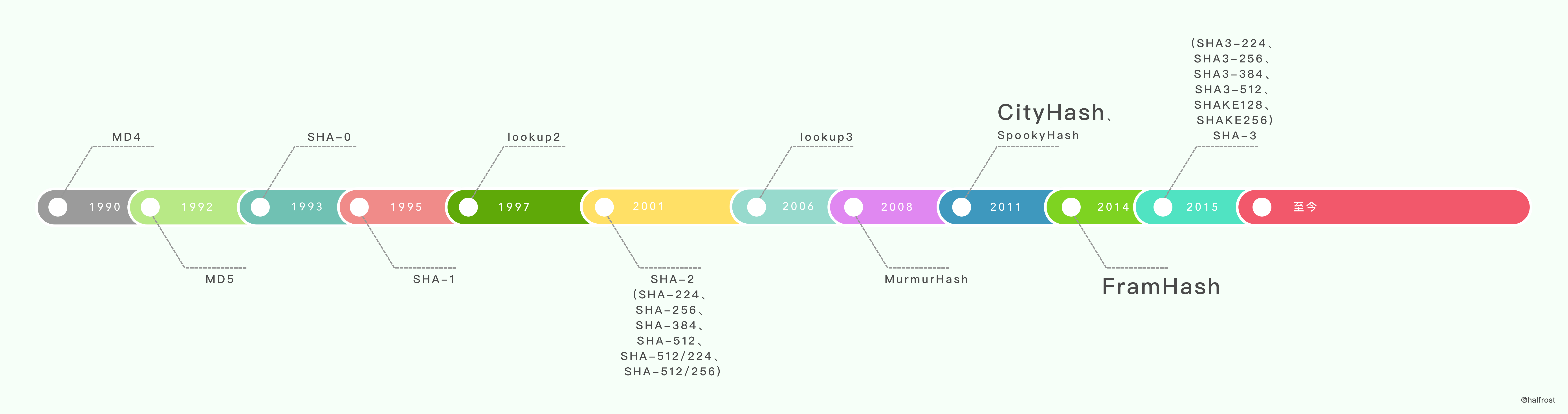
Both of these algorithms are string algorithms released by Google.
CityHash is a string hashing algorithm released by Google in 2011. Like MurmurHash, it is a non-cryptographic hash algorithm. The development of CityHash was inspired by MurmurHash. Its main advantage is that most steps contain at least two independent mathematical operations. Modern CPUs can usually achieve optimal performance from this kind of code. CityHash also has its drawbacks: the code is more complex than comparable popular algorithms. Google wanted to optimize for speed rather than simplicity, so it did not add special cases for shorter inputs. Google released two algorithms: cityhash64 and cityhash128. They compute 64-bit and 128-bit hash values for strings, respectively. These algorithms are not suitable for cryptography, but are appropriate for use in hash tables and similar scenarios. CityHash’s speed depends on the CRC32 instruction, currently SSE 4.2 (Intel Nehalem and later).
Compared with MurmurHash, which supports 32-, 64-, and 128-bit hashes, CityHash supports 64-, 128-, and 256-bit hashes.
In 2014, Google released FarmHash, a new family of hash functions for strings. FarmHash inherits many techniques and tricks from CityHash and is its successor. FarmHash has multiple goals and claims to improve on CityHash in several respects. Another improvement over CityHash is that FarmHash provides a single interface on top of multiple platform-specific implementations. This means that when developers simply want a fast, robust hash function for a hash table, without requiring identical behavior on every platform, FarmHash can satisfy that requirement as well. Currently, FarmHash only includes hash functions for byte arrays on 32-, 64-, and 128-bit platforms. Future development plans include support for integers, tuples, and other data.
(4) xxHash
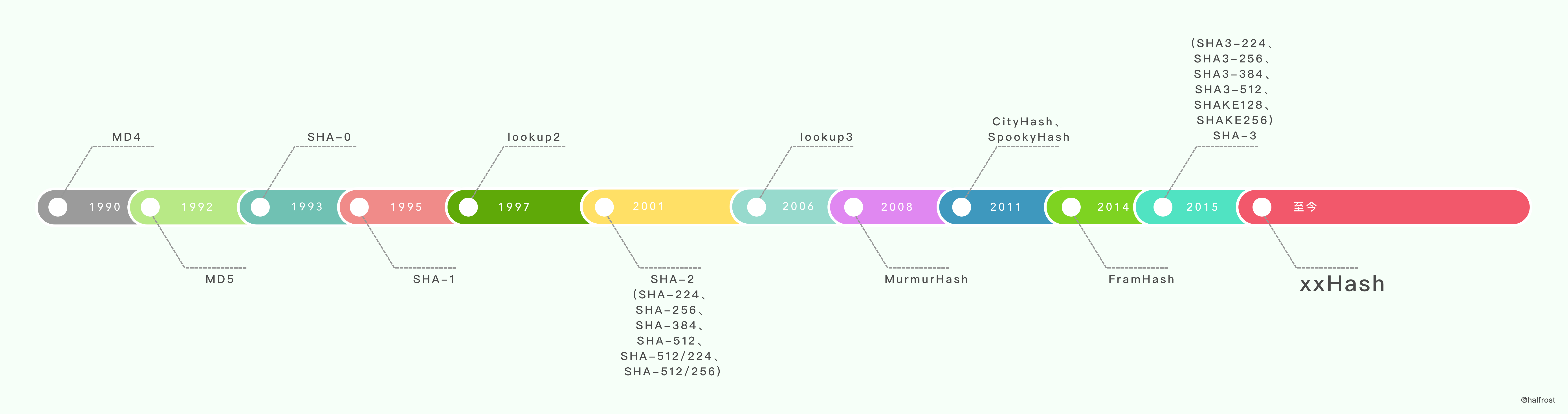
xxHash is a non-cryptographic hash function created by Yann Collet. It was originally used in the LZ4 compression algorithm as the final error-checking signature. The speed of this hash algorithm approaches the limits of RAM. It provides both 32-bit and 64-bit versions. Today, it is widely used in databases such as PrestoDB, RocksDB, MySQL, ArangoDB, PGroonga, and Spark, and also in game frameworks such as Cocos2D, Dolphin, and Cxbx-reloaded.
Below is a performance comparison experiment. The test environment is the Open-Source SMHasher program by Austin Appleby , compiled with Visual C on Windows 7, and it uses only a single thread. The CPU core is a Core 2 Duo @3.0GHz.
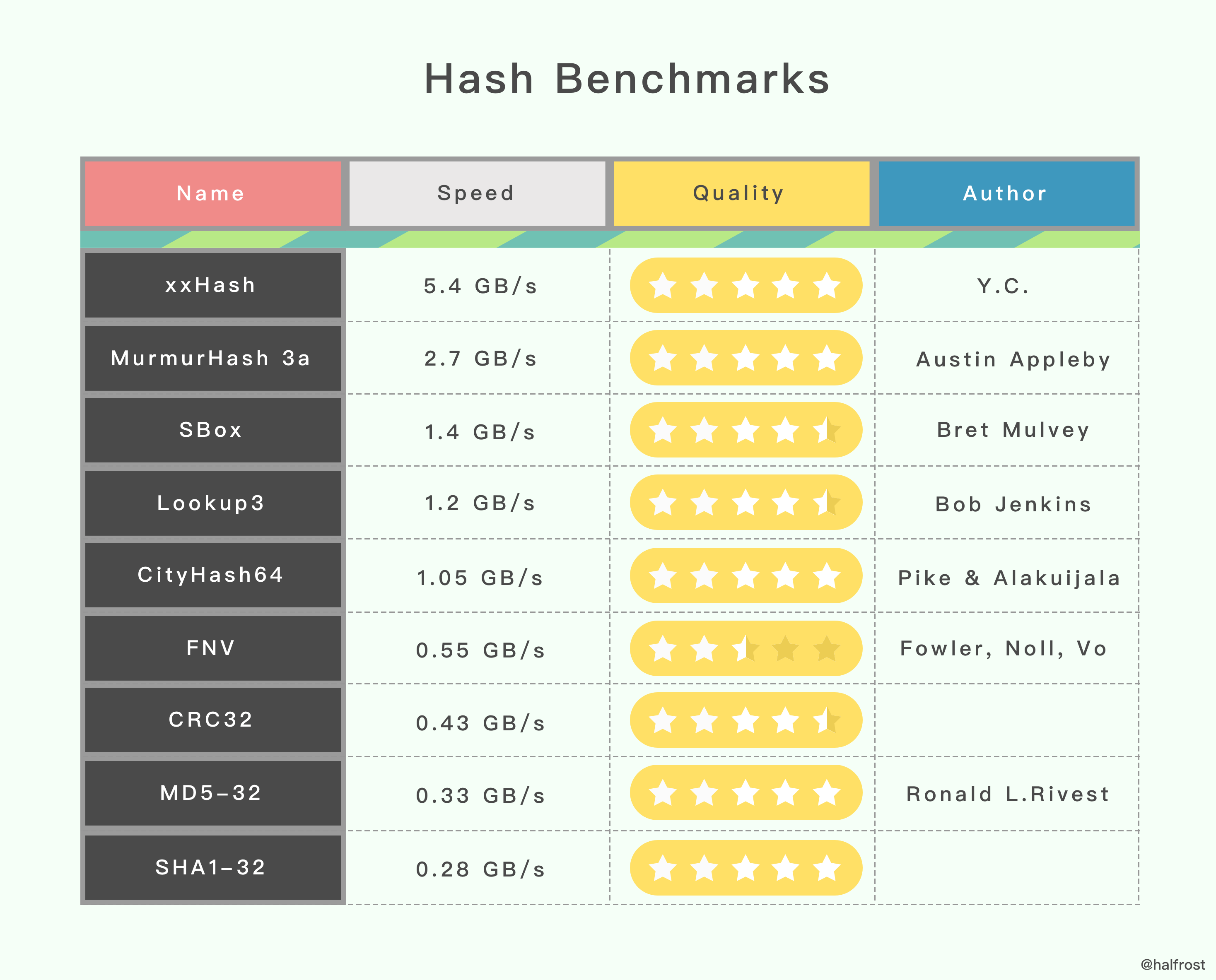
The hash functions in the table above are not all existing hash functions; it only lists some common algorithms. The second column compares speed, and you can see that xxHash is the fastest. The third column is hash quality. There are five algorithms with the highest hash quality, all rated five stars: xxHash, MurmurHash 3a, CityHash64, MD5-32, and SHA1-32. Judging from the data in the table, the hash function with both the highest quality and the fastest speed is still xxHash.
(4) memhash
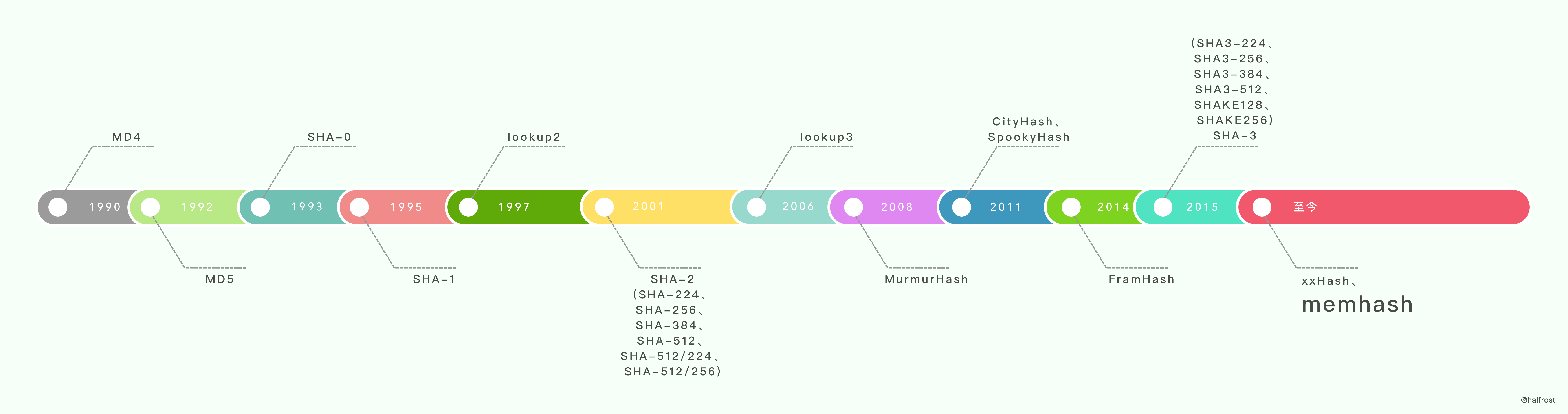
The author was unable to find very clear information online about the author of this hashing algorithm. There are only a few lines of comments in Google’s Go documentation indicating its source of inspiration:
// Hashing algorithm inspired by
//   xxhash: https://code.google.com/p/xxhash/
// cityhash: https://code.google.com/p/cityhash/
It says memhash was inspired by xxhash and cityhash. Next, let’s look at how memhash hashes strings.
const (
	// Constants for multiplication: four random odd 32-bit numbers.
	m1 = 3168982561
	m2 = 3339683297
	m3 = 832293441
	m4 = 2336365089
)

func memhash(p unsafe.Pointer, seed, s uintptr) uintptr {
	if GOARCH == "386" && GOOS != "nacl" && useAeshash {
		return aeshash(p, seed, s)
	}
	h := uint32(seed + s*hashkey[0])
tail:
	switch {
	case s == 0:
	case s < 4:
		h ^= uint32(*(*byte)(p))
		h ^= uint32(*(*byte)(add(p, s>>1))) << 8
		h ^= uint32(*(*byte)(add(p, s-1))) << 16
		h = rotl_15(h*m1) * m2
	case s == 4:
		h ^= readUnaligned32(p)
		h = rotl_15(h*m1) * m2
	case s <= 8:
		h ^= readUnaligned32(p)
		h = rotl_15(h*m1) * m2
		h ^= readUnaligned32(add(p, s-4))
		h = rotl_15(h*m1) * m2
	case s <= 16:
		h ^= readUnaligned32(p)
		h = rotl_15(h*m1) * m2
		h ^= readUnaligned32(add(p, 4))
		h = rotl_15(h*m1) * m2
		h ^= readUnaligned32(add(p, s-8))
		h = rotl_15(h*m1) * m2
		h ^= readUnaligned32(add(p, s-4))
		h = rotl_15(h*m1) * m2
	default:
		v1 := h
		v2 := uint32(seed * hashkey[1])
		v3 := uint32(seed * hashkey[2])
		v4 := uint32(seed * hashkey[3])
		for s >= 16 {
			v1 ^= readUnaligned32(p)
			v1 = rotl_15(v1*m1) * m2
			p = add(p, 4)
			v2 ^= readUnaligned32(p)
			v2 = rotl_15(v2*m2) * m3
			p = add(p, 4)
			v3 ^= readUnaligned32(p)
			v3 = rotl_15(v3*m3) * m4
			p = add(p, 4)
			v4 ^= readUnaligned32(p)
			v4 = rotl_15(v4*m4) * m1
			p = add(p, 4)
			s -= 16
		}
		h = v1 ^ v2 ^ v3 ^ v4
		goto tail
	}
	h ^= h >> 17
	h *= m3
	h ^= h >> 13
	h *= m4
	h ^= h >> 16
	return uintptr(h)
}

// Note: in order to get the compiler to issue rotl instructions, we
// need to constant fold the shift amount by hand.
// TODO: convince the compiler to issue rotl instructions after inlining.
func rotl_15(x uint32) uint32 {
	return (x << 15) | (x >> (32 - 15))
}
m1, m2, m3, and m4 are four randomly selected odd numbers used as multiplication factors in the hash.
// used in hash{32,64}.go to seed the hash function
var hashkey [4]uintptr

func alginit() {
	// Install aes hash algorithm if we have the instructions we need
	if (GOARCH == "386" || GOARCH == "amd64") &&
		GOOS != "nacl" &&
		cpuid_ecx&(1<<25) != 0 && // aes (aesenc)
		cpuid_ecx&(1<<9) != 0 && // sse3 (pshufb)
		cpuid_ecx&(1<<19) != 0 { // sse4.1 (pinsr{d,q})
		useAeshash = true
		algarray[alg_MEM32].hash = aeshash32
		algarray[alg_MEM64].hash = aeshash64
		algarray[alg_STRING].hash = aeshashstr
		// Initialize with random data so hash collisions will be hard to engineer.
		getRandomData(aeskeysched[:])
		return
	}
	getRandomData((*[len(hashkey) * sys.PtrSize]byte)(unsafe.Pointer(&hashkey))[:])
	hashkey[0] |= 1 // make sure these numbers are odd
	hashkey[1] |= 1
	hashkey[2] |= 1
	hashkey[3] |= 1
}
In this initialization function, two arrays are initialized, both filled with random hash keys. On 386, amd64, non-NaCl platforms, aeshash is used. Here, random keys are generated and stored in the aeskeysched array. Similarly, four random numbers are generated for the hashkey array as well. Finally, the low bit is forced to 1 to ensure that the generated random numbers are all odd.
Next, let’s look at an example to see exactly how memhash computes a hash value.
func main() {
	r := [8]byte{'h', 'a', 'l', 'f', 'r', 'o', 's', 't'}
	pp := memhashpp(unsafe.Pointer(&r), 3, 7)
	fmt.Println(pp)
}
For simplicity, we’ll use the author’s name as an example to compute the hash value, and set the seed to a simple value of 3.
The first step is to compute the value of h.
h := uint32(seed + s*hashkey[0])
Assume here that hashkey[0] = 1, then the value of h is 3 + 7 * 1 = 10. Since s < 8, the following processing will be performed:
    case s <= 8:
        h ^= readUnaligned32(p)
        h = rotl_15(h*m1) * m2
        h ^= readUnaligned32(add(p, s-4))
        h = rotl_15(h*m1) * m2
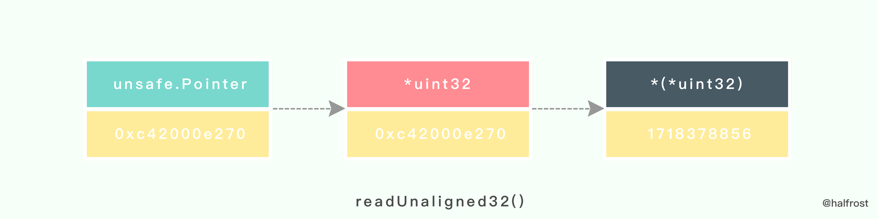
The readUnaligned32() function converts the incoming unsafe.Pointer pointer twice: first to the *uint32 type, and then to the *(*uint32) type.
Next, it performs an XOR operation:
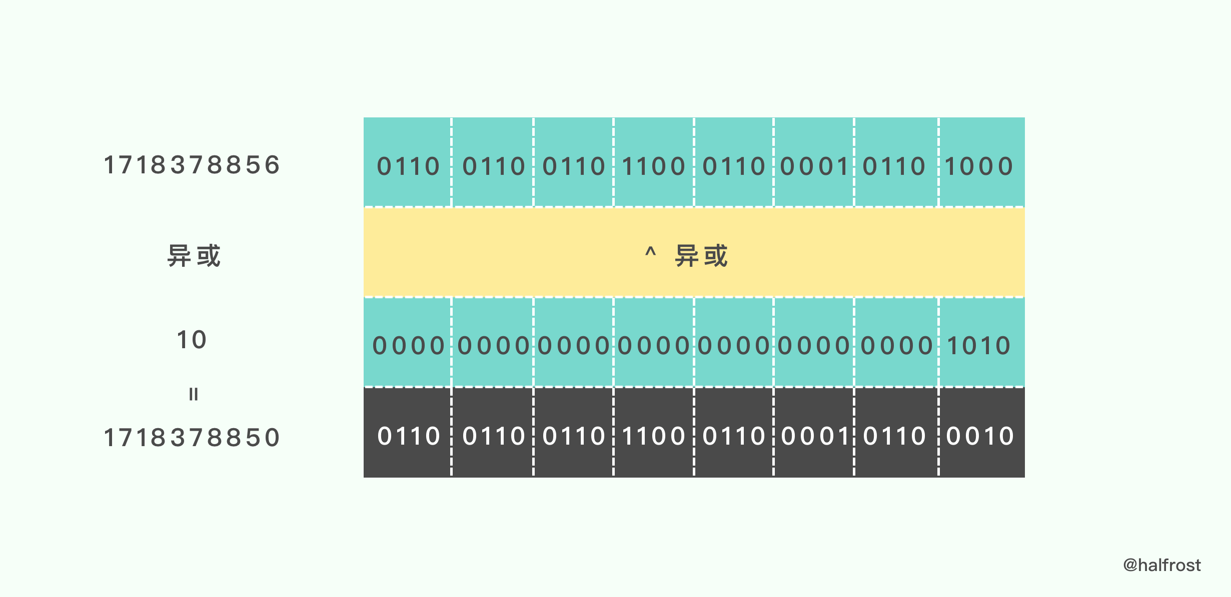
Then the second step is h * m1 = 1718378850 * 3168982561 = 3185867170
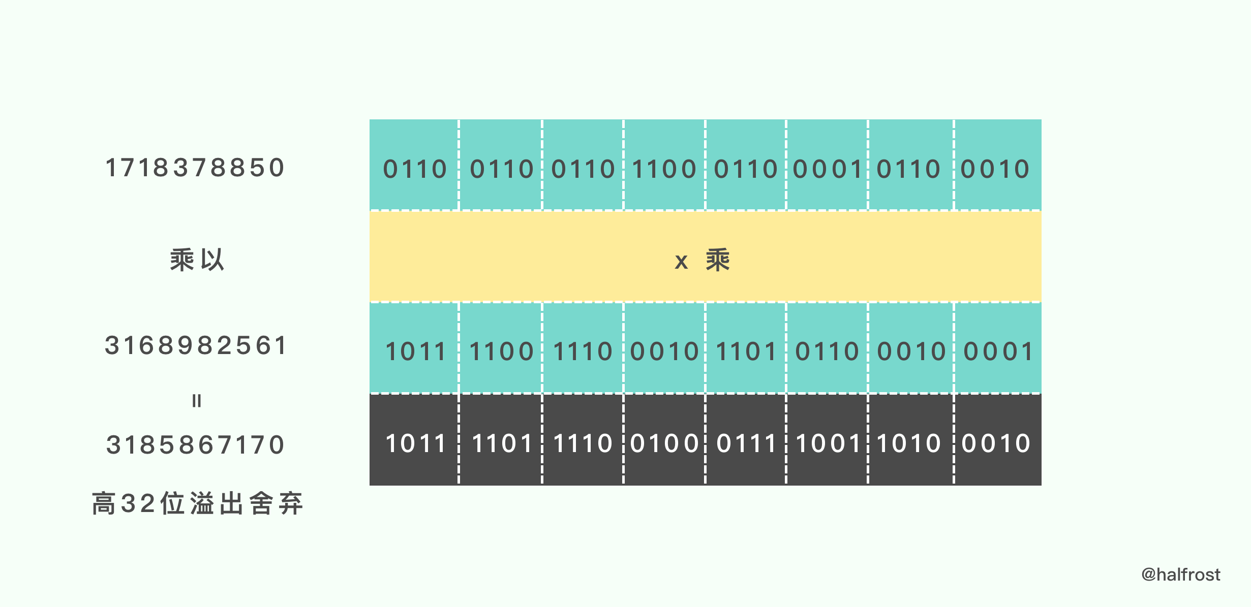
Because this is 32-bit multiplication, the final result is 64 bits; the high 32 bits overflow and are discarded directly.
The multiplication result is used as the input to rotl_15().
func rotl_15(x uint32) uint32 {
	return (x << 15) | (x >> (32 - 15))
}
This function performs two bit-shift operations on the input parameters.
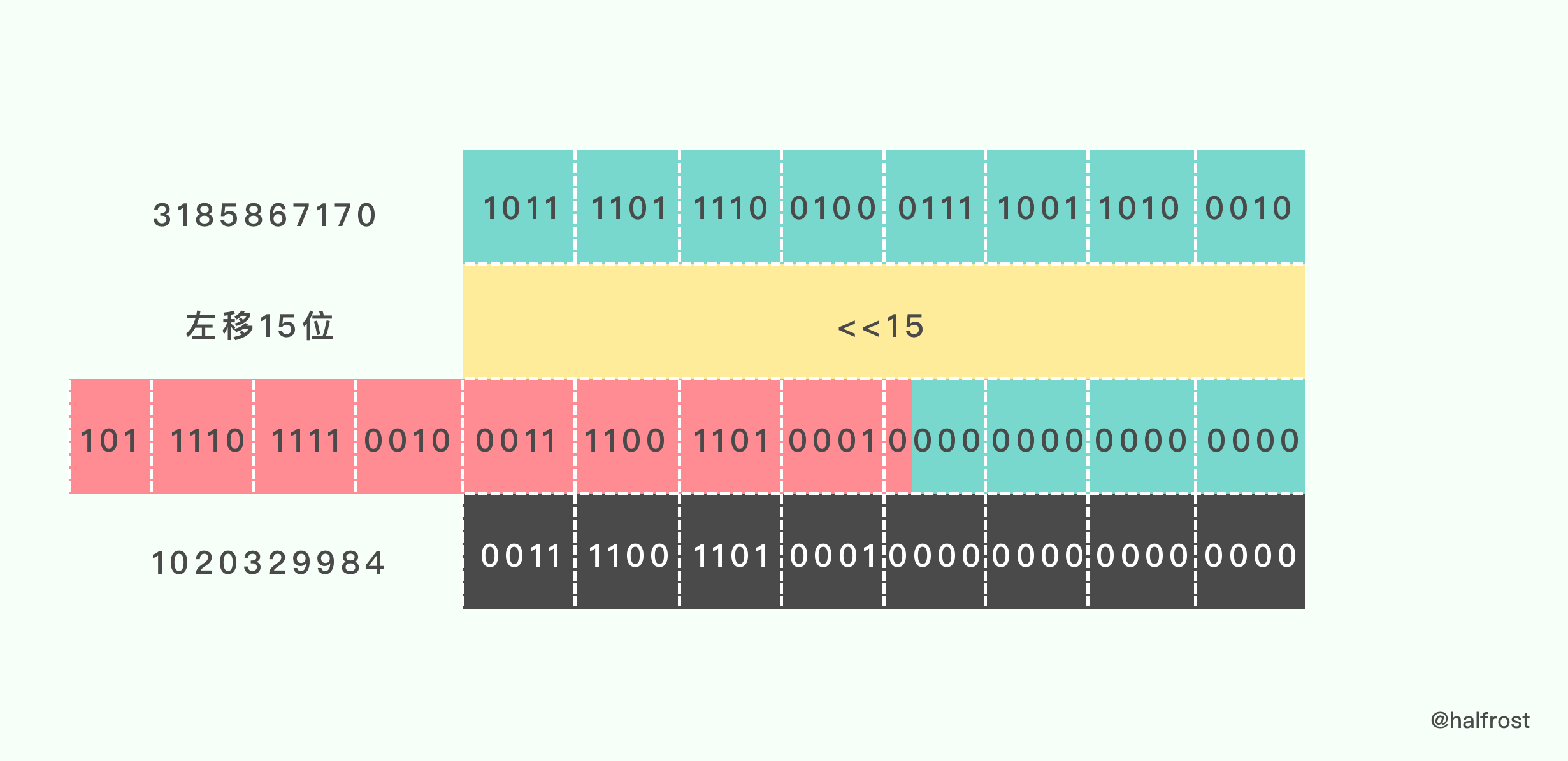
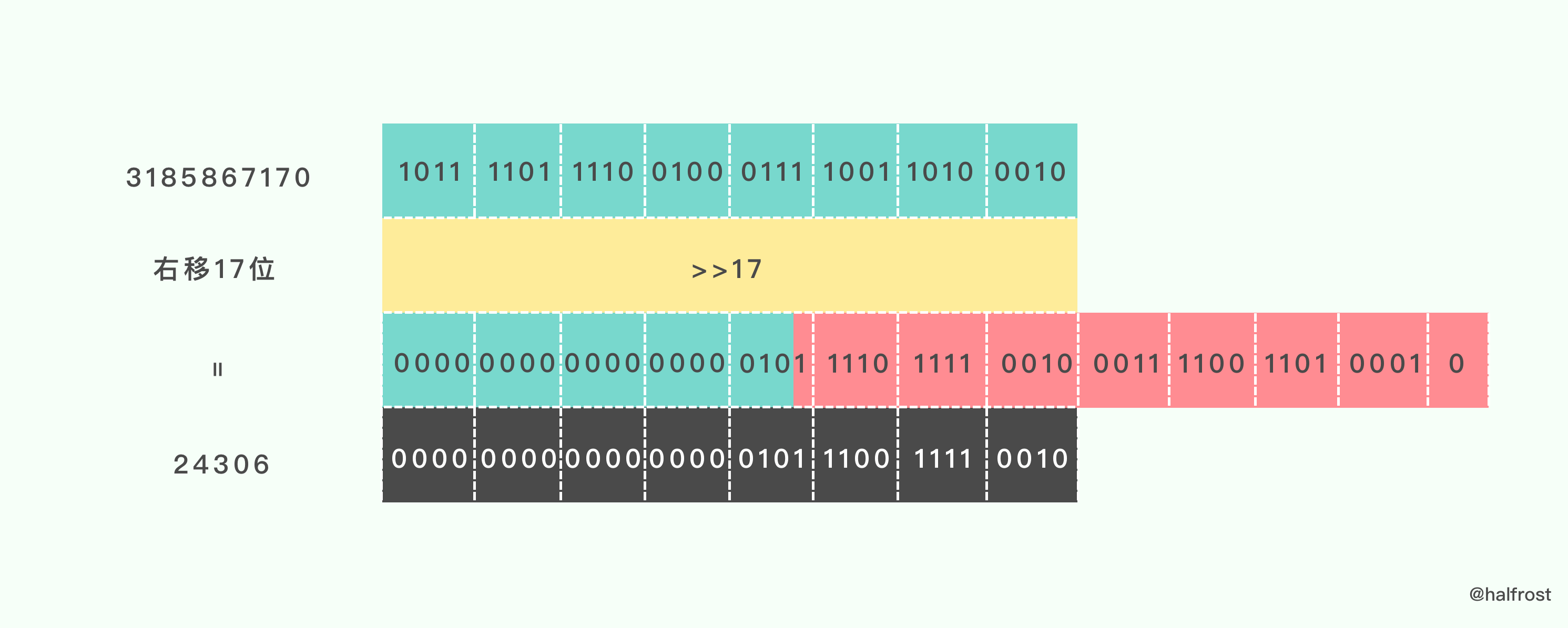
Finally, it performs a logical OR operation on the results of the two shifts:
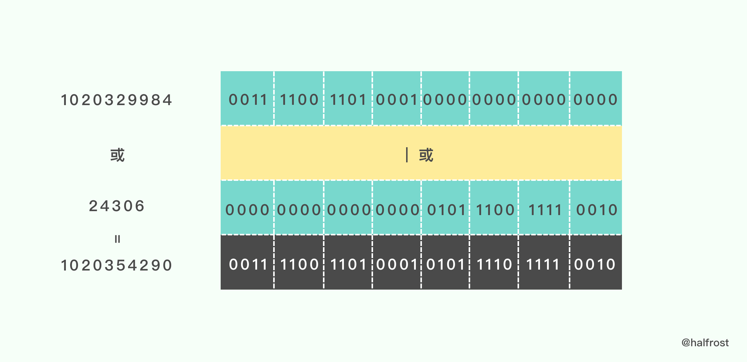
Then it performs another readUnaligned32() conversion:
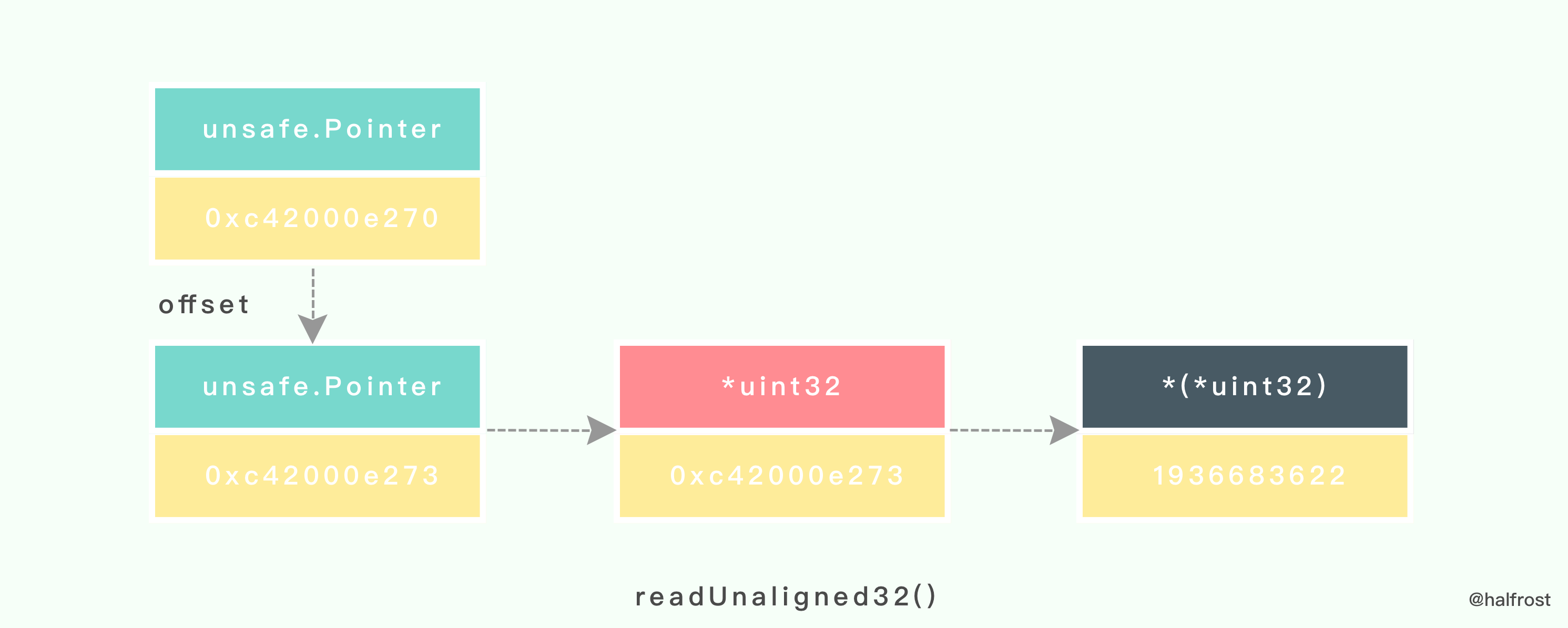
After the conversion, it performs another XOR. At this point, h = 2615762644.
Then it also needs to perform another rotl_15() transformation. I won’t illustrate that with a diagram here. After the transformation is complete, h = 2932930721.
Finally, execute the last step of the hash:
    h ^= h >> 17
    h *= m3
    h ^= h >> 13
    h *= m4
    h ^= h >> 16
Right-shift by 17 bits, then XOR, then multiply by m3, then right-shift by 13 bits, then XOR, then multiply by m4, then right-shift by 16 bits, and finally XOR again.
After this series of operations, the hash value is produced. The final value is h = 1870717864. Interested readers can work through the calculation themselves.
(5) AES Hash
When analyzing Go’s hash algorithm above, we saw that it checks whether the CPU supports the AES instruction set. If the CPU supports the AES instruction set, it uses the AES Hash algorithm; if not, it falls back to the memhash algorithm.
The full name of the AES instruction set is the Advanced Encryption Standard instruction set (also known as Intel Advanced Encryption Standard New Instructions, abbreviated as AES-NI). It is an extension to the x86 instruction set architecture, used by Intel and AMD microprocessors.
Implementing a hash algorithm with AES can deliver excellent performance because it provides hardware acceleration.
The concrete implementation is shown below. It is assembly code; see the comments in the program below:
// aes hash algorithm implemented using AES hardware instructions
TEXT runtime·aeshash(SB),NOSPLIT,$0-32
	MOVQ	p+0(FP), AX	// move ptr to the data segment
	MOVQ	s+16(FP), CX	// length
	LEAQ	ret+24(FP), DX
	JMP	runtime·aeshashbody(SB)

TEXT runtime·aeshashstr(SB),NOSPLIT,$0-24
	MOVQ	p+0(FP), AX	// move ptr to the string struct
	MOVQ	8(AX), CX	// string length
	MOVQ	(AX), AX	// string data
	LEAQ	ret+16(FP), DX
	JMP	runtime·aeshashbody(SB)
The actual hash implementation is all in aeshashbody:
// AX: data
// CX: length
// DX: return address
TEXT runtime·aeshashbody(SB),NOSPLIT,$0-0
	// Load our random seed into SSE registers
	MOVQ	h+8(FP), X0			// The hash seed in each table is 64 bits
	PINSRW	$4, CX, X0			// Length takes 16 bits
	PSHUFHW $0, X0, X0			// Shuffle high words, repeat length 4 times
	MOVO	X0, X1				// Save the seed before encryption
	PXOR	runtime·aeskeysched(SB), X0	// XOR each seed being processed
	AESENC	X0, X0				// Encrypt the seed

	CMPQ	CX, $16
	JB	aes0to15
	JE	aes16
	CMPQ	CX, $32
	JBE	aes17to32
	CMPQ	CX, $64
	JBE	aes33to64
	CMPQ	CX, $128
	JBE	aes65to128
	JMP	aes129plus

// aes from 0 - 15
aes0to15:
	TESTQ	CX, CX
	JE	aes0

	ADDQ	$16, AX
	TESTW	$0xff0, AX
	JE	endofpage

	//The address of the 16 bytes being loaded will not cross a page boundary, so we can load it directly.
	MOVOU	-16(AX), X1
	ADDQ	CX, CX
	MOVQ	$masks<>(SB), AX
	PAND	(AX)(CX*8), X1
final1:
	PXOR	X0, X1	// XOR data and seed
	AESENC	X1, X1	// Encrypt 3 times in a row
	AESENC	X1, X1
	AESENC	X1, X1
	MOVQ	X1, (DX)
	RET

endofpage:
	// The address ends with 1111xxxx. This may cross a page boundary, so stop loading after the last byte. Then use pshufb to shift the bytes down.
	MOVOU	-32(AX)(CX*1), X1
	ADDQ	CX, CX
	MOVQ	$shifts<>(SB), AX
	PSHUFB	(AX)(CX*8), X1
	JMP	final1

aes0:
	// Return the input seed after encryption
	AESENC	X0, X0
	MOVQ	X0, (DX)
	RET

aes16:
	MOVOU	(AX), X1
	JMP	final1

aes17to32:
	// Start processing the second initial seed
	PXOR	runtime·aeskeysched+16(SB), X1
	AESENC	X1, X1

	// Load the data to be processed by the hash algorithm
	MOVOU	(AX), X2
	MOVOU	-16(AX)(CX*1), X3

	// XOR the seeds
	PXOR	X0, X2
	PXOR	X1, X3

	// Encrypt 3 times in a row
	AESENC	X2, X2
	AESENC	X3, X3
	AESENC	X2, X2
	AESENC	X3, X3
	AESENC	X2, X2
	AESENC	X3, X3

	// Combine and generate the result
	PXOR	X3, X2
	MOVQ	X2, (DX)
	RET

aes33to64:
	// Process the third and later initial seeds
	MOVO	X1, X2
	MOVO	X1, X3
	PXOR	runtime·aeskeysched+16(SB), X1
	PXOR	runtime·aeskeysched+32(SB), X2
	PXOR	runtime·aeskeysched+48(SB), X3
	AESENC	X1, X1
	AESENC	X2, X2
	AESENC	X3, X3

	MOVOU	(AX), X4
	MOVOU	16(AX), X5
	MOVOU	-32(AX)(CX*1), X6
	MOVOU	-16(AX)(CX*1), X7

	PXOR	X0, X4
	PXOR	X1, X5
	PXOR	X2, X6
	PXOR	X3, X7

	AESENC	X4, X4
	AESENC	X5, X5
	AESENC	X6, X6
	AESENC	X7, X7

	AESENC	X4, X4
	AESENC	X5, X5
	AESENC	X6, X6
	AESENC	X7, X7

	AESENC	X4, X4
	AESENC	X5, X5
	AESENC	X6, X6
	AESENC	X7, X7

	PXOR	X6, X4
	PXOR	X7, X5
	PXOR	X5, X4
	MOVQ	X4, (DX)
	RET

aes65to128:
	// Process the seventh and later initial seeds
	MOVO	X1, X2
	MOVO	X1, X3
	MOVO	X1, X4
	MOVO	X1, X5
	MOVO	X1, X6
	MOVO	X1, X7
	PXOR	runtime·aeskeysched+16(SB), X1
	PXOR	runtime·aeskeysched+32(SB), X2
	PXOR	runtime·aeskeysched+48(SB), X3
	PXOR	runtime·aeskeysched+64(SB), X4
	PXOR	runtime·aeskeysched+80(SB), X5
	PXOR	runtime·aeskeysched+96(SB), X6
	PXOR	runtime·aeskeysched+112(SB), X7
	AESENC	X1, X1
	AESENC	X2, X2
	AESENC	X3, X3
	AESENC	X4, X4
	AESENC	X5, X5
	AESENC	X6, X6
	AESENC	X7, X7

	// Load data
	MOVOU	(AX), X8
	MOVOU	16(AX), X9
	MOVOU	32(AX), X10
	MOVOU	48(AX), X11
	MOVOU	-64(AX)(CX*1), X12
	MOVOU	-48(AX)(CX*1), X13
	MOVOU	-32(AX)(CX*1), X14
	MOVOU	-16(AX)(CX*1), X15

	// XOR the seeds
	PXOR	X0, X8
	PXOR	X1, X9
	PXOR	X2, X10
	PXOR	X3, X11
	PXOR	X4, X12
	PXOR	X5, X13
	PXOR	X6, X14
	PXOR	X7, X15

	// Encrypt 3 times in a row
	AESENC	X8, X8
	AESENC	X9, X9
	AESENC	X10, X10
	AESENC	X11, X11
	AESENC	X12, X12
	AESENC	X13, X13
	AESENC	X14, X14
	AESENC	X15, X15

	AESENC	X8, X8
	AESENC	X9, X9
	AESENC	X10, X10
	AESENC	X11, X11
	AESENC	X12, X12
	AESENC	X13, X13
	AESENC	X14, X14
	AESENC	X15, X15

	AESENC	X8, X8
	AESENC	X9, X9
	AESENC	X10, X10
	AESENC	X11, X11
	AESENC	X12, X12
	AESENC	X13, X13
	AESENC	X14, X14
	AESENC	X15, X15

	// Assemble the result
	PXOR	X12, X8
	PXOR	X13, X9
	PXOR	X14, X10
	PXOR	X15, X11
	PXOR	X10, X8
	PXOR	X11, X9
	PXOR	X9, X8
	MOVQ	X8, (DX)
	RET

aes129plus:
	// Process the seventh and later initial seeds
	MOVO	X1, X2
	MOVO	X1, X3
	MOVO	X1, X4
	MOVO	X1, X5
	MOVO	X1, X6
	MOVO	X1, X7
	PXOR	runtime·aeskeysched+16(SB), X1
	PXOR	runtime·aeskeysched+32(SB), X2
	PXOR	runtime·aeskeysched+48(SB), X3
	PXOR	runtime·aeskeysched+64(SB), X4
	PXOR	runtime·aeskeysched+80(SB), X5
	PXOR	runtime·aeskeysched+96(SB), X6
	PXOR	runtime·aeskeysched+112(SB), X7
	AESENC	X1, X1
	AESENC	X2, X2
	AESENC	X3, X3
	AESENC	X4, X4
	AESENC	X5, X5
	AESENC	X6, X6
	AESENC	X7, X7

	// Start in reverse order, from the last block, because overlap may occur
	MOVOU	-128(AX)(CX*1), X8
	MOVOU	-112(AX)(CX*1), X9
	MOVOU	-96(AX)(CX*1), X10
	MOVOU	-80(AX)(CX*1), X11
	MOVOU	-64(AX)(CX*1), X12
	MOVOU	-48(AX)(CX*1), X13
	MOVOU	-32(AX)(CX*1), X14
	MOVOU	-16(AX)(CX*1), X15

	// XOR the seeds
	PXOR	X0, X8
	PXOR	X1, X9
	PXOR	X2, X10
	PXOR	X3, X11
	PXOR	X4, X12
	PXOR	X5, X13
	PXOR	X6, X14
	PXOR	X7, X15

	// Compute the number of remaining 128-byte blocks
	DECQ	CX
	SHRQ	$7, CX

aesloop:
	// Encrypt state
	AESENC	X8, X8
	AESENC	X9, X9
	AESENC	X10, X10
	AESENC	X11, X11
	AESENC	X12, X12
	AESENC	X13, X13
	AESENC	X14, X14
	AESENC	X15, X15

	// Encrypt state within the same block and XOR
	MOVOU	(AX), X0
	MOVOU	16(AX), X1
	MOVOU	32(AX), X2
	MOVOU	48(AX), X3
	AESENC	X0, X8
	AESENC	X1, X9
	AESENC	X2, X10
	AESENC	X3, X11
	MOVOU	64(AX), X4
	MOVOU	80(AX), X5
	MOVOU	96(AX), X6
	MOVOU	112(AX), X7
	AESENC	X4, X12
	AESENC	X5, X13
	AESENC	X6, X14
	AESENC	X7, X15

	ADDQ	$128, AX
	DECQ	CX
	JNE	aesloop

	// Final step: perform 3 or more encryptions
	AESENC	X8, X8
	AESENC	X9, X9
	AESENC	X10, X10
	AESENC	X11, X11
	AESENC	X12, X12
	AESENC	X13, X13
	AESENC	X14, X14
	AESENC	X15, X15
	AESENC	X8, X8
	AESENC	X9, X9
	AESENC	X10, X10
	AESENC	X11, X11
	AESENC	X12, X12
	AESENC	X13, X13
	AESENC	X14, X14
	AESENC	X15, X15
	AESENC	X8, X8
	AESENC	X9, X9
	AESENC	X10, X10
	AESENC	X11, X11
	AESENC	X12, X12
	AESENC	X13, X13
	AESENC	X14, X14
	AESENC	X15, X15

	PXOR	X12, X8
	PXOR	X13, X9
	PXOR	X14, X10
	PXOR	X15, X11
	PXOR	X10, X8
	PXOR	X11, X9
	PXOR	X9, X8
	MOVQ	X8, (DX)
	RET
2. Handling Hash Collisions
(1) Array of Linked Lists
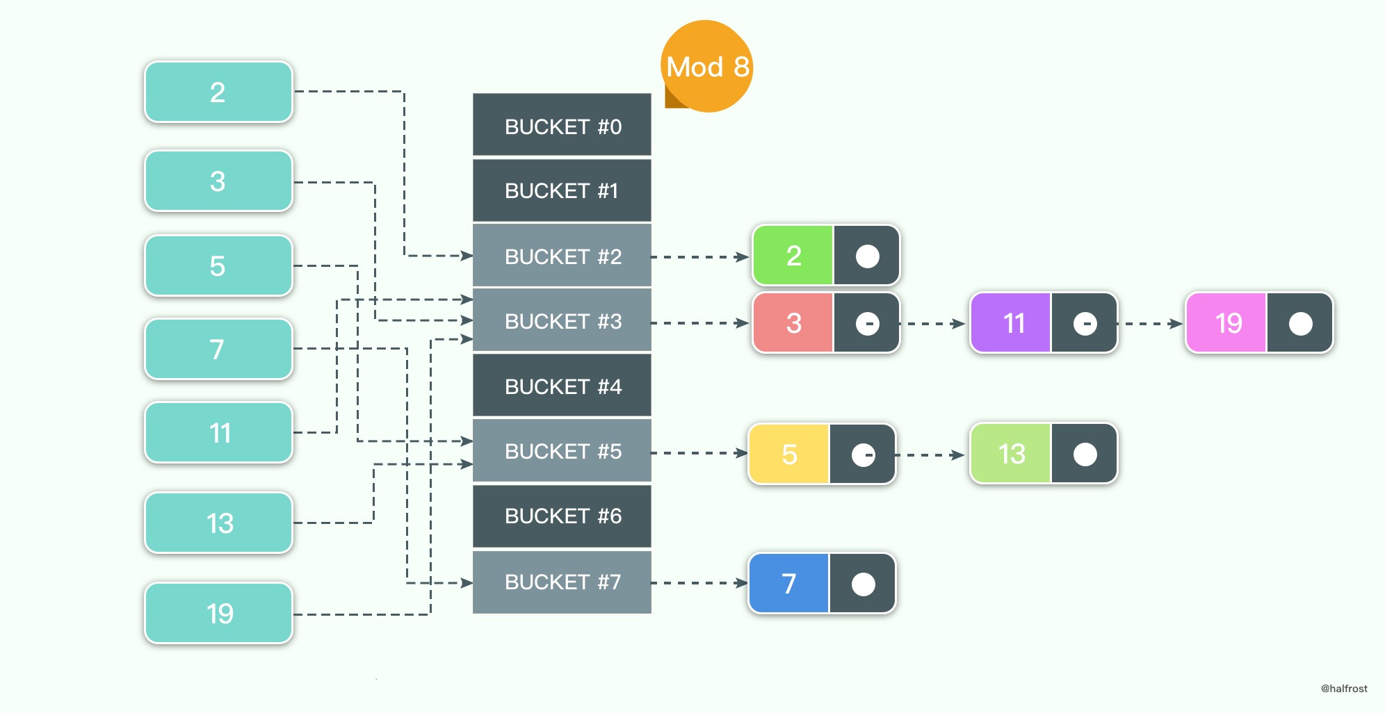
The array-of-linked-lists approach is relatively simple: take each key-value pair modulo the table length; if the result is the same, insert it sequentially into a linked list.
Suppose the set of keys to be inserted is {2, 3, 5, 7, 11, 13, 19}, and the table length is MOD 8. Assume the hash function is uniformly distributed over [0, 9), as shown above.
Next, focus on the performance analysis:
When looking up a key k, assume key k is not in the hash table and h(k) is uniformly distributed over [0, M), that is, P(h(k) = i) = 1/M. Let Xi be the number of keys contained in ht[ i ]. If h(k) = i, then the number of key comparisons for an unsuccessful lookup of k is Xi. Therefore:

The analysis for successful lookups is slightly more complex. We need to consider the order in which entries are added to the hash table. Ignoring the case of duplicate keys, assume K = {k1, k2, …… kn}, and assume the keys are inserted into an initially empty hash table in this order. Introduce a random variable: if h(ki) = h(kj), then Xij = 1; if h(ki) != h(kj), then Xij = 0.
Because of the previous assumption that the hash table is uniformly distributed, P(Xij = i) = E(Xij) = 1/M, where E(X) denotes the mathematical expectation of random variable X. Further assume that each key is added to the end of the linked list. Let Ci be the number of key comparisons needed to find Ki. Since the probability of looking up Ki cannot be determined in advance, assume that the probability of looking up each key is the same, namely 1/n. Then we have:
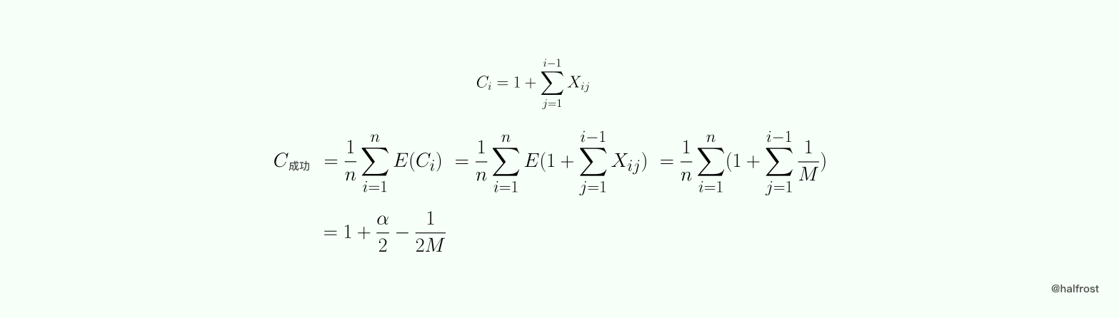
From this we can see that the performance of a hash table has little to do with the number of elements in the table, and is instead related to the load factor α. If the hash table length is proportional to the number of elements in the hash table, then the complexity of hash table lookup is O(1).
In summary, the average number of key comparisons for successful and unsuccessful lookups in an array of linked lists is as follows:

(2) Open Addressing — Linear Probing
The rule for linear probing is hi = ( h(k) + i ) MOD M. For example, i = 1, M = 9.
With this collision-handling method, once a collision occurs, the position is incremented by 1 until an empty position is found.
For example, suppose the set of keys to be inserted is {2, 3, 5, 7, 11, 13, 19}, and the value added after a collision in linear probing is 1. The final result is as follows:
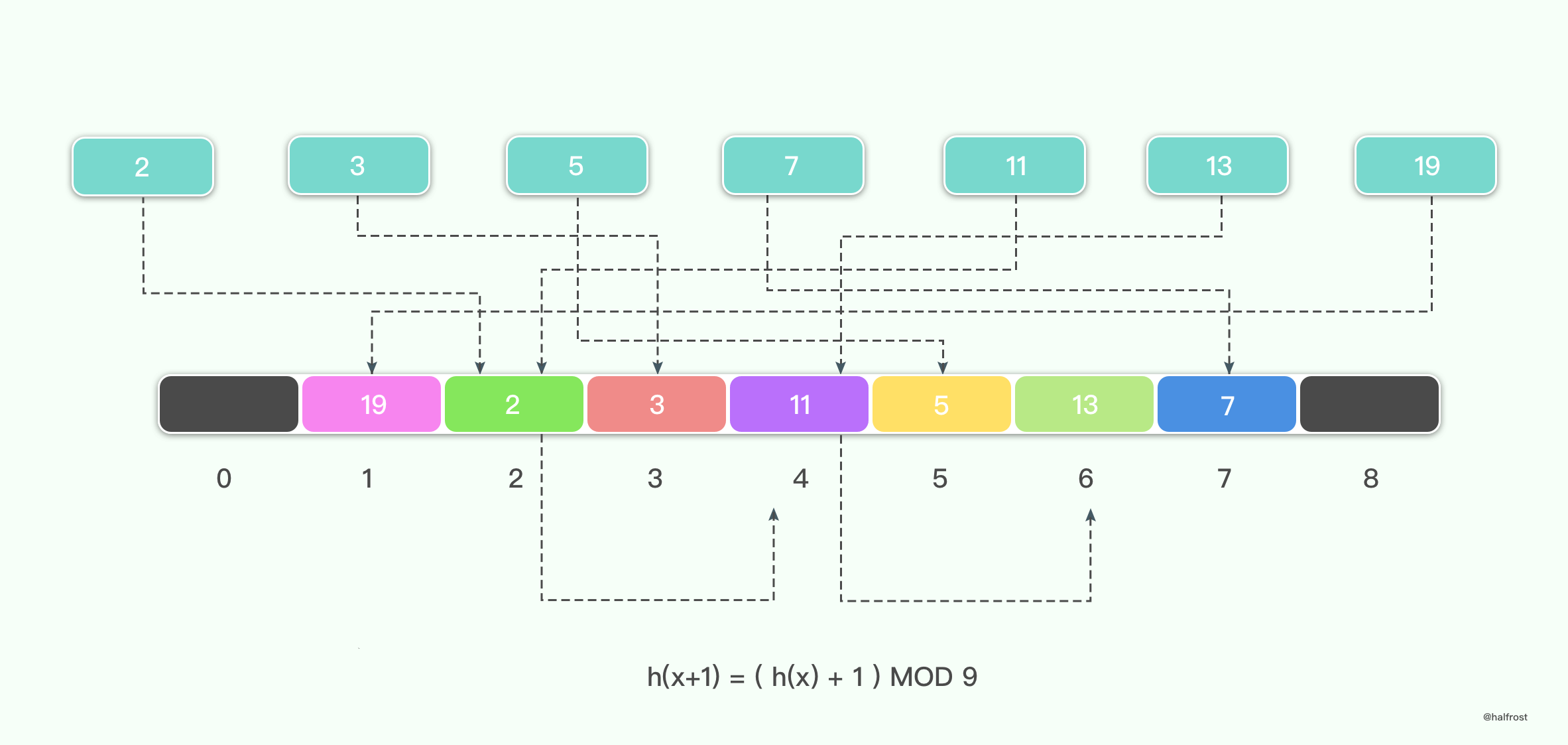
The performance analysis of linear-probing hash tables is relatively complex, so only the result is given here.

(3) Open Addressing — Quadratic Probing
The rule for linear probing is h0 = h(k), hi = ( h0 + i * i ) MOD M.
For example, suppose the set of keys to be inserted is {2, 3, 5, 7, 11, 13, 20}, and the value added after a collision in quadratic probing is the square of the number of probes. The final result is as follows:
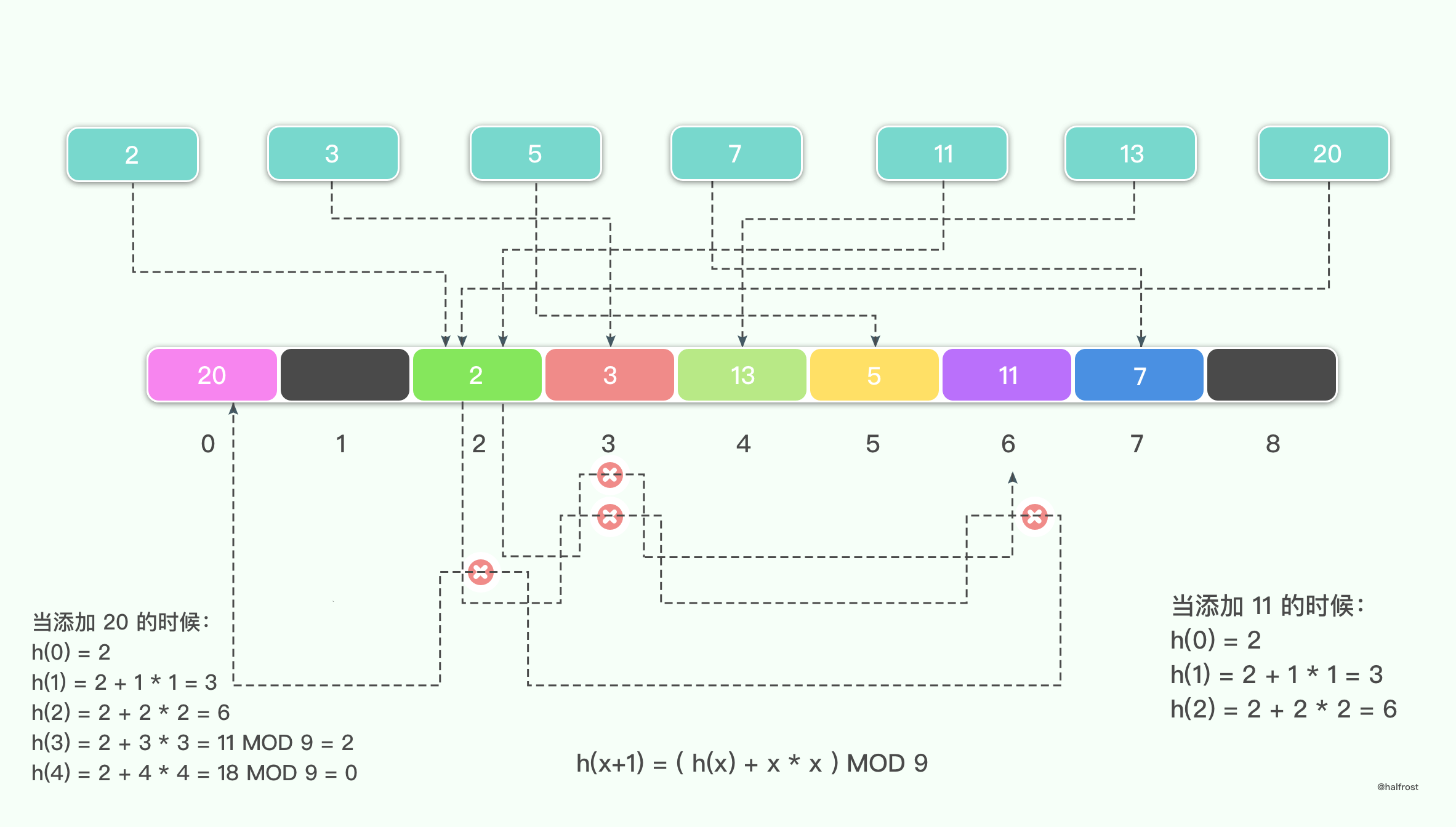
Quadratic probing adds a quadratic curve on top of linear probing. After a collision occurs, instead of adding a linear parameter, it adds the square of the number of probes.
One thing to note about quadratic probing is that the size of M matters. If M is not an odd prime, the following problem may occur: even if there are still empty positions in the hash table, an element may still fail to find a position to insert into.
For example, suppose M = 10 and the set of keys to be inserted is {0, 1, 4, 5, 6, 9, 10}. After the first six keys have been inserted into the hash table, 10 can no longer be inserted.
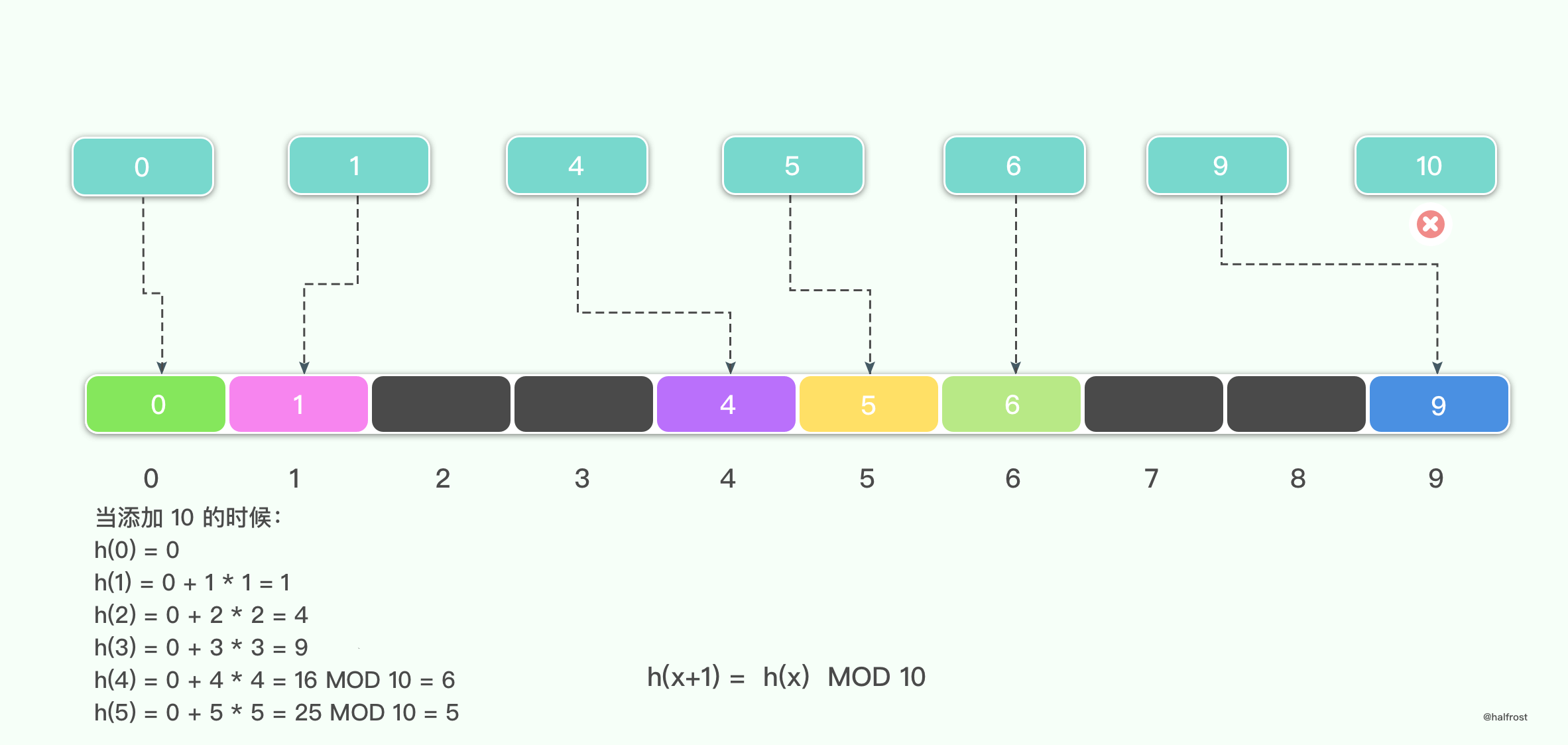
Therefore, in quadratic probing, the following rule holds:
If M is an odd prime, then the following ⌈M / 2⌉ positions h0, h1, h2 …… h⌊M/2⌋ are all distinct. Here, hi = (h0 + i * i ) MOD M.
This rule can be proved by contradiction. Suppose hi = hj, i > j; 0<=i, j<= ⌊M/2⌋. Then h0 + i* i = ( h0 + j * j ) MOD M, so M can divide ( i + j )( i - j ). Since M is prime and 0 < i + j, i - j < M, this can hold if and only if i = j.
The above rule also shows that as long as M is an odd prime, quadratic probing can traverse at least half of the positions in the hash table. Therefore, as long as the load factor α <= 1 / 2, quadratic probing can always find an insertable position.
In the example above, the reason key 10 cannot be inserted is also because α > 1 / 2, so an insertable position can no longer be guaranteed.
(4) Open Addressing — Double Hashing
Double hashing is intended to address clustering. Whether with linear probing or quadratic probing, if h(k1) and h(k2) are adjacent, their probe sequences will also be adjacent. This is the so-called clustering phenomenon. To avoid this, a second hash function h2 is introduced so that the distance between two probes is h2(k). Thus the probe sequence is h0 = h1(k), hi = ( h0 + i * h2(k) ) MOD M. Experiments show that the performance of double hashing is similar to random probing.
Analyzing the average search length of double hashing and quadratic probing is more difficult than for linear probing. Therefore, the concept of random probing is introduced to approximate these two probing strategies. Random probing means that the probe sequence { hi } is selected independently and uniformly at random from the interval [0, M], so P(hi = j) = 1/M.
Assume the probe sequence is h0, h1, ……, hi. The position hi in the hash table is empty, while the positions h0, h1, ……, hi-1 are not empty. The number of key comparisons for this lookup is i. Let the random variable X be the number of key comparisons required for an unsuccessful lookup. Since the load factor of the hash table is α, the probability that a position in the hash table is empty is 1 - α, and the probability that it is non-empty is α. Therefore, P( X = i ) = α^i * ( 1 - α ).
In probability theory, the above distribution is called the geometric distribution.

Assume the insertion order of elements into the hash table is {k1, k2, …… , kn}. Let Xi be the number of key comparisons for an unsuccessful lookup when the hash table contains only {k1, k2, …… , ki}. Note that at this point the load factor of the hash table is i/M, so the number of key comparisons to find k(i+1) is Yi = 1 + Xi. Assuming the probability of looking up any key is 1/n, the average number of key comparisons for a successful lookup is:

In summary, the average number of key comparisons for successful and unsuccessful lookups with quadratic probing and double hashing is as follows:

Overall, when the data volume is very large, simple hash functions inevitably produce collisions. Even if an appropriate collision-handling method is used, there is still a certain time complexity. Therefore, if you want to avoid collisions as much as possible, you should choose a high-performance hash function, or increase the number of hash bits, such as 64-bit, 128-bit, or 256-bit, which makes the probability of collisions much lower.
3. Hash Table Resizing Strategy
As the load factor of a hash table increases, the number of collisions also increases, and the performance of the hash table becomes worse and worse. For hash tables implemented with separate chaining, this may still be tolerable, but for open addressing, such a performance degradation is unacceptable. Therefore, for open addressing, we need to find a way to solve this problem.
In practice, the solution is to dynamically increase the length of the hash table. When the load factor exceeds a certain threshold, the length of the hash table is increased automatically. Whenever the length of the hash table changes, the index corresponding to every key in the hash table must be recomputed; entries cannot simply be copied from the original hash table into the new hash table. The hash value of each key in the original hash table must be computed one by one and inserted into the new hash table. This approach clearly cannot meet production requirements, because its time complexity is too high: O(n). Once the data volume becomes large, performance will be poor. Redis came up with a method that allows an insert operation to be completed in constant time O(1) even when growth is triggered. The solution is to copy the old hash table into the new hash table incrementally over multiple steps, rather than completing the copy all at once.
Next, using Redis as an example, let’s discuss how its hash table resizes without significantly affecting performance.
Redis defines a dictionary as follows:
/*
 * Dictionary
 *
 * Each dictionary uses two hash tables to implement incremental rehashing
 */
typedef struct dict {
    // Type-specific handler functions
    dictType *type;
    // Private data for type handler functions
    void *privdata;
    // Hash tables (2)
    dictht ht[2];
    // Flag recording rehash progress; -1 means rehashing is not in progress
    int rehashidx;
    // Number of safe iterators currently active
    int iterators;
} dict;
From the definition, we can see that a Redis dictionary maintains two hash tables, and the hash table ht[1] is used for rehashing.
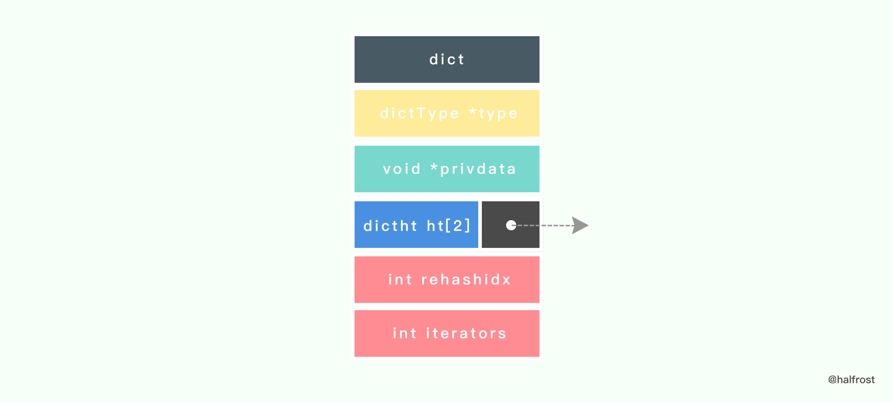
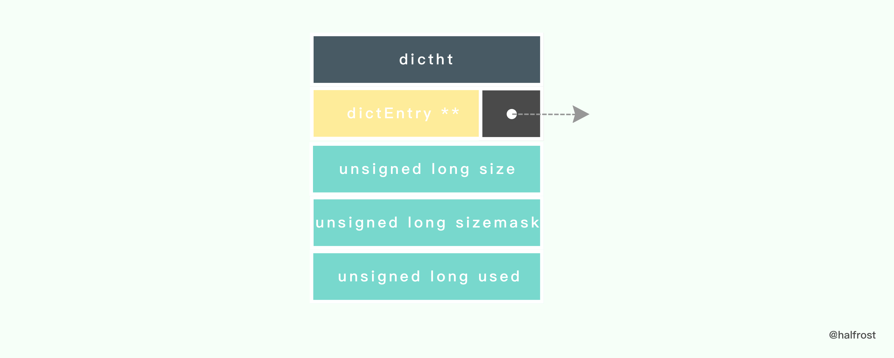
Redis defines the hash table data structure as follows:
/*
 * Hash table
 */
typedef struct dictht {
    // Array of hash table node pointers (commonly called buckets)
    dictEntry **table;
    // Size of the pointer array
    unsigned long size;
    // Length mask of the pointer array, used to compute index values
    unsigned long sizemask;
    // Current number of nodes in the hash table
    unsigned long used;

} dictht;
The table attribute is an array, and each element of the array is a pointer to a dictEntry structure.
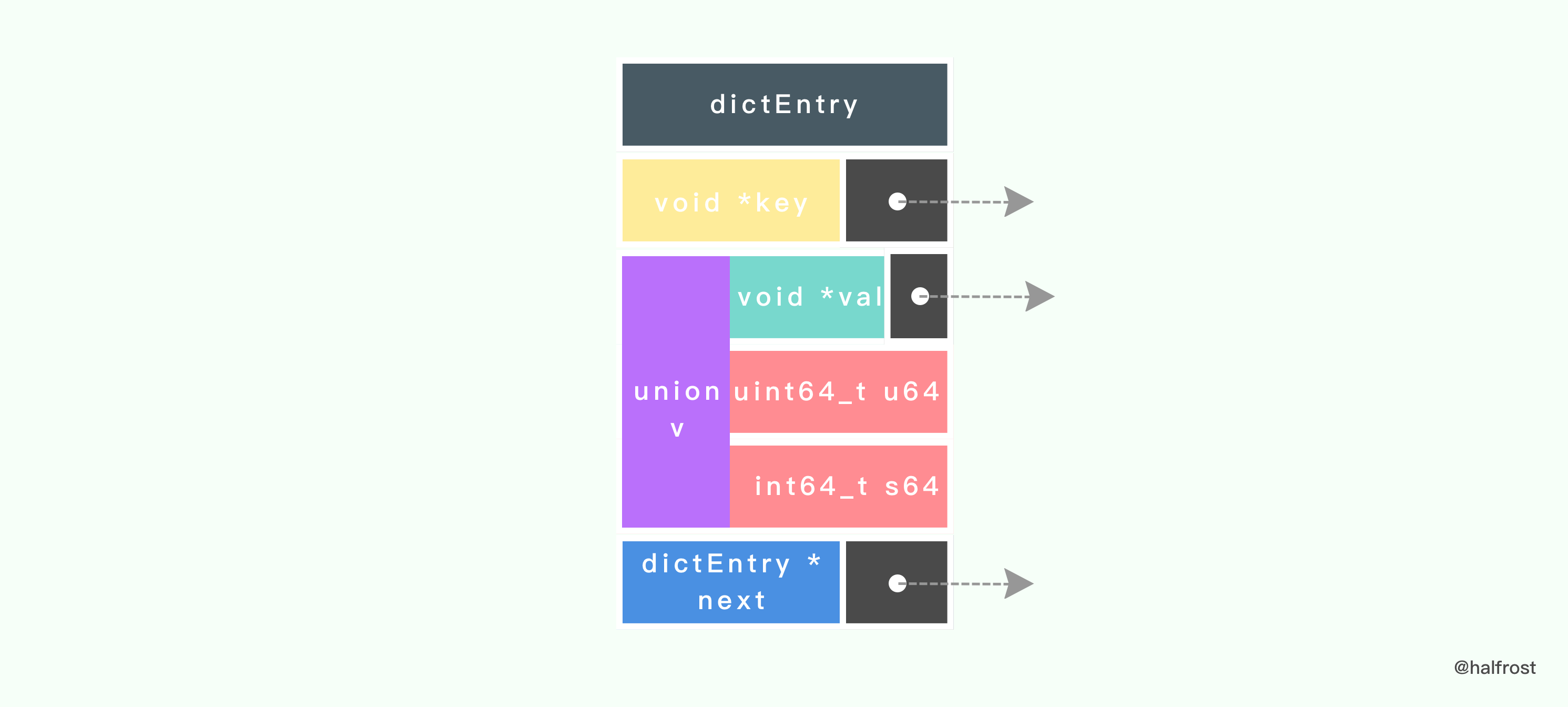
Each dictEntry stores a key-value pair, as well as a pointer to another dictEntry structure:
/*
 * Hash table node
 */
typedef struct dictEntry {
    // Key
    void *key;
    // Value
    union {
        void *val;
        uint64_t u64;
        int64_t s64;
    } v;
    // Link to the next node
    struct dictEntry *next;

} dictEntry;
The next field points to another dictEntry structure. Multiple dictEntry instances can be linked together into a linked list through the next pointer. From this, we can see that dictht uses separate chaining to handle key collisions.
Before adding a new key-value pair to the dictionary, dictAdd checks hash table ht[0]. For the size and used fields of ht[0], if the ratio ratio = used / size satisfies either of the following conditions, the rehash process is activated:
Natural rehash: ratio >= 1, and the variable dict_can_resize is true.
Forced rehash: ratio is greater than the variable dict_force_resize_ratio (in the current version, the value of dict_force_resize_ratio is 5).
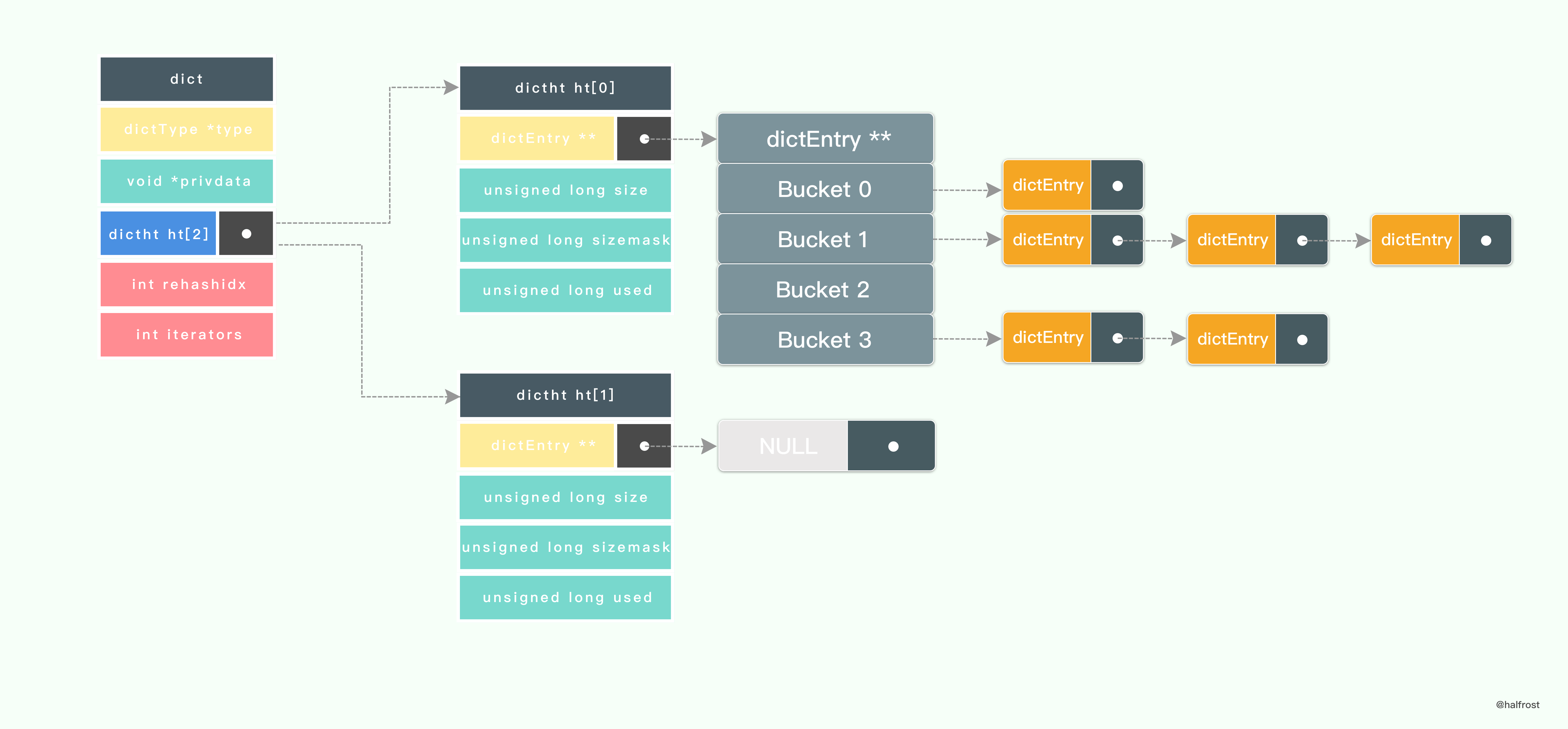
Assume the current dictionary needs to be expanded and rehashed. Redis first sets the dictionary’s rehashidx to 0, marking the start of rehashing; then it allocates space for ht[1]->table, with a size of at least twice ht[0]->used.
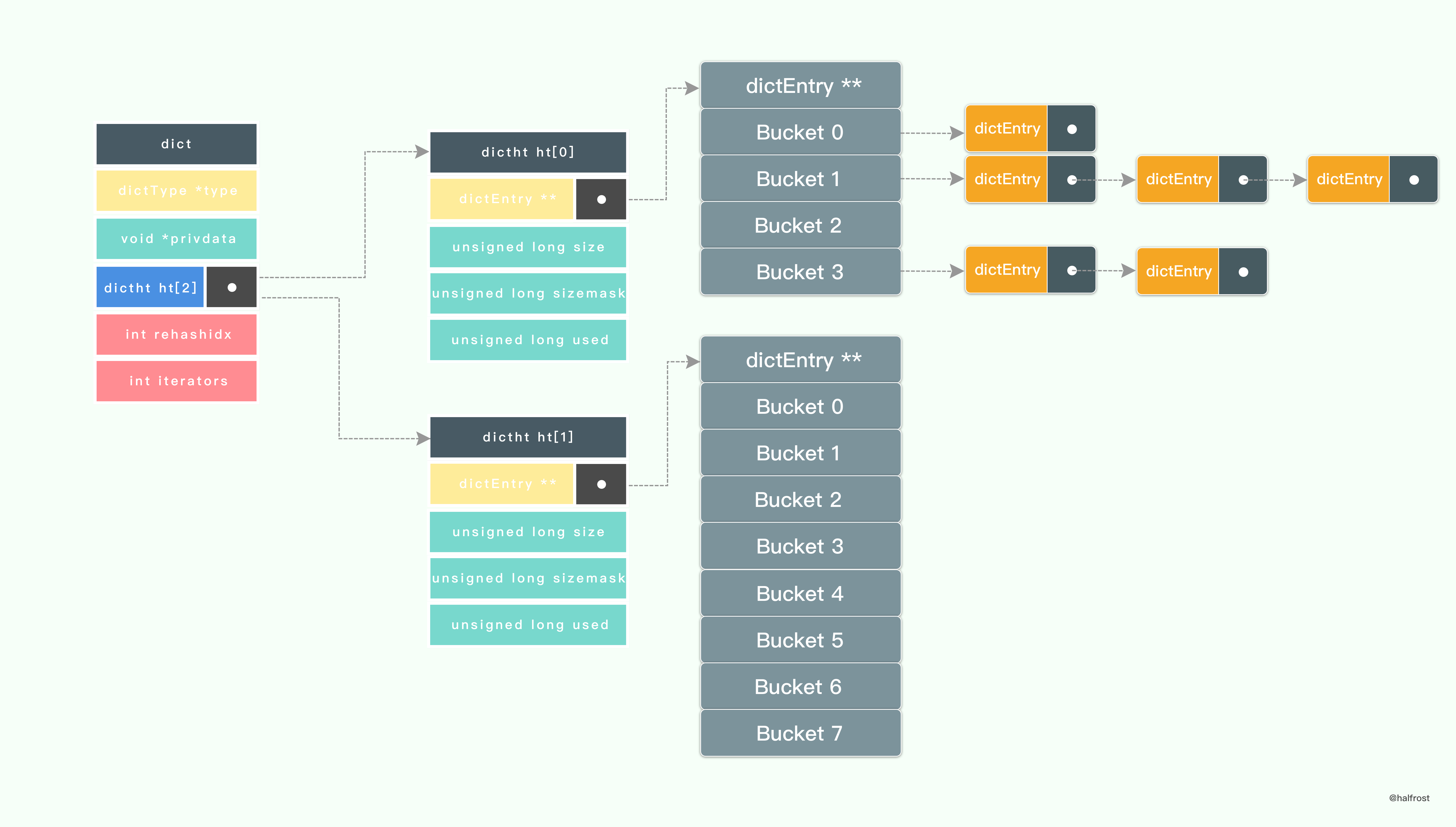
As shown above, space for 8 slots has already been allocated for ht[1]->table.
Next, rehashing begins. The key-value pairs in ht[0]->table are moved into ht[1]->table. This movement is not completed all at once, but is performed incrementally over multiple steps.
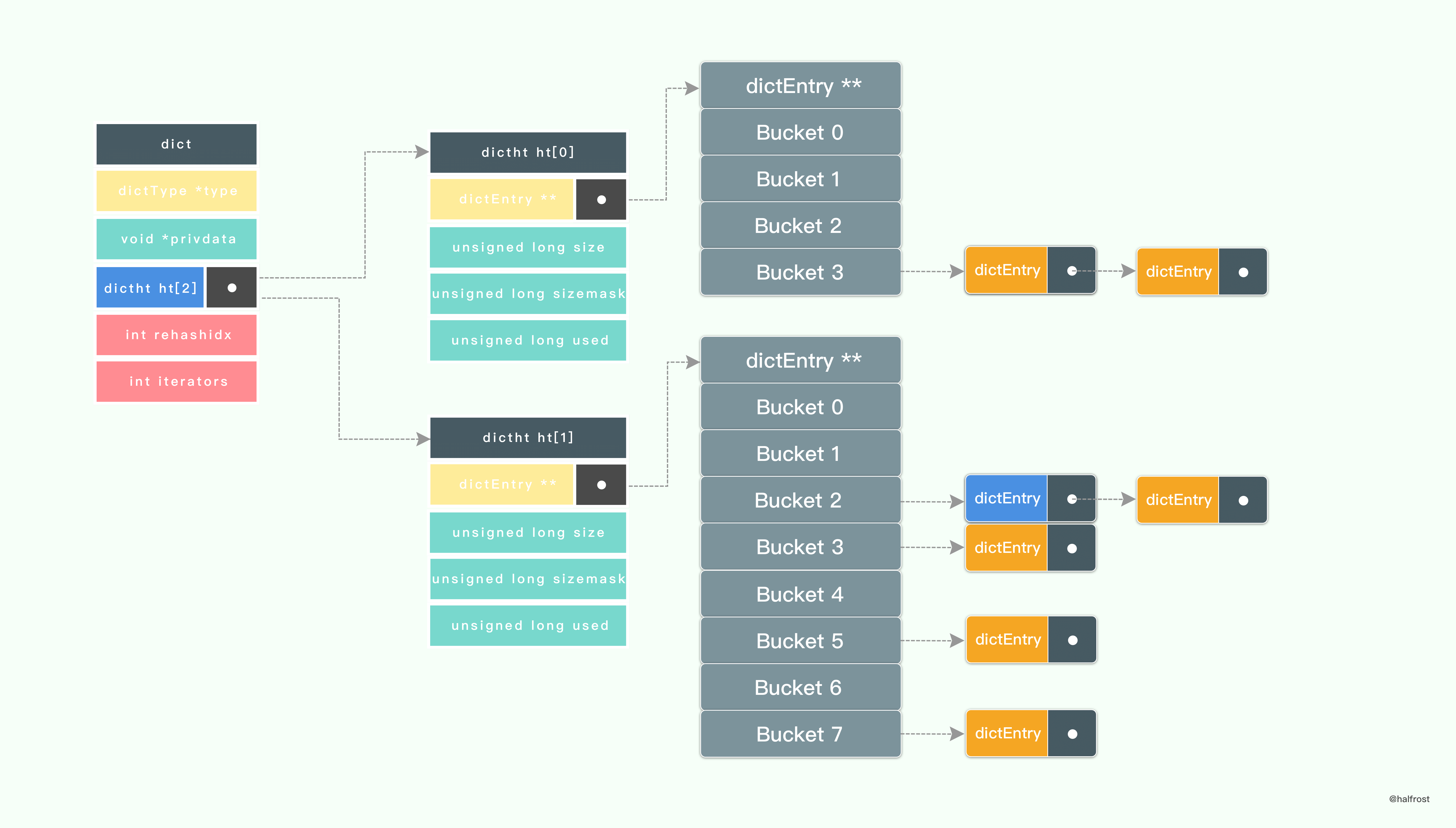
As shown above, some key-value pairs in ht[0] have already been migrated to ht[1]. At this point, new key-value pairs may also be inserted, and they are inserted directly into ht[1] rather than ht[0]. This ensures that ht[0] only decreases and never increases.
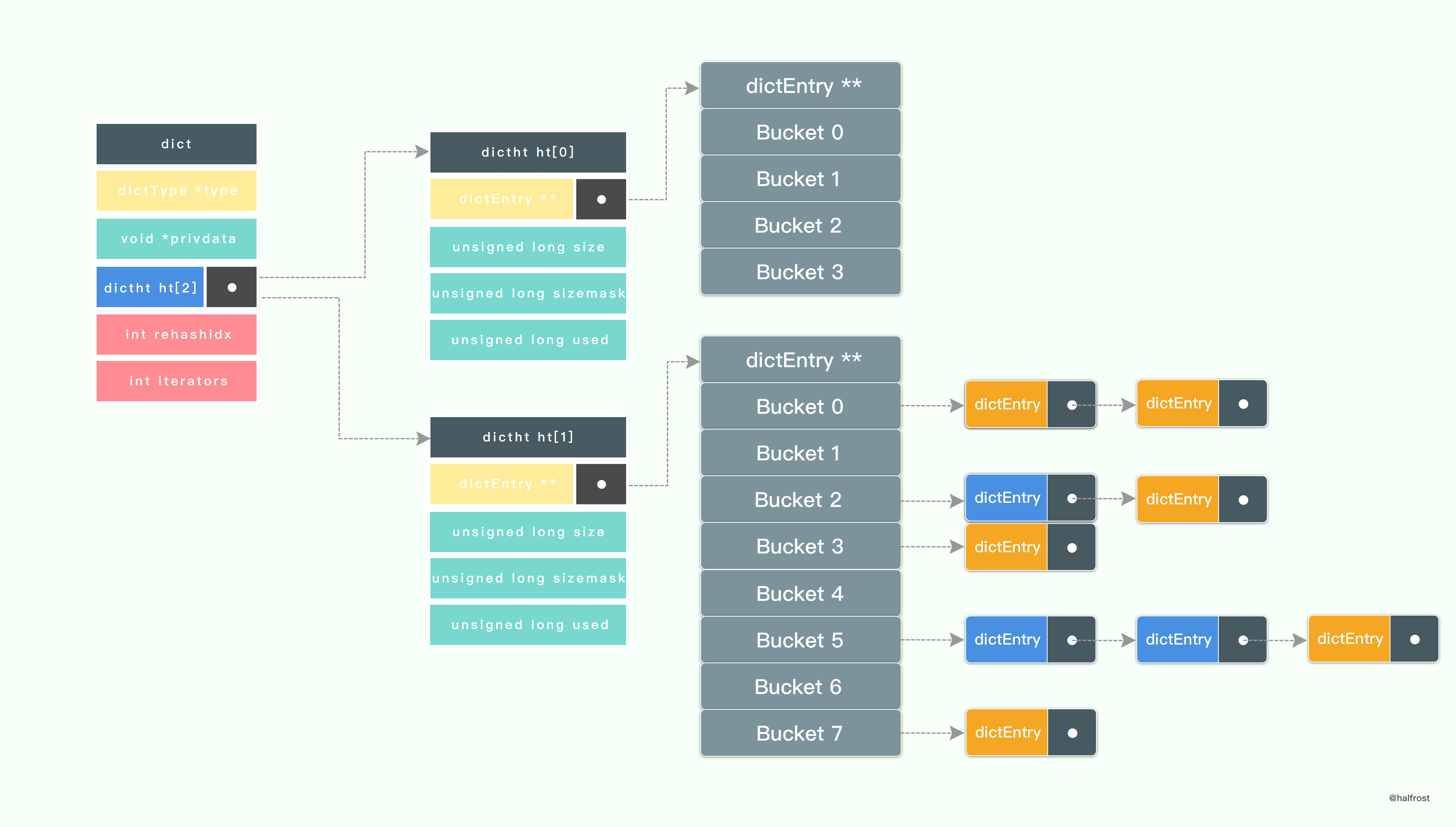
During the rehash process, new key-value pairs continue to be inserted, while the key-value pairs in ht[0] continue to be migrated over, until all key-value pairs in ht[0] have been migrated. Note that Redis uses head insertion: new values are always inserted at the first position of the linked list. This avoids traversing to the end of the list and saves the O(n) time complexity. By the time the process reaches the state shown above, all nodes have been migrated.
Before rehashing ends, cleanup is performed: the space used by ht[0] is released; ht[1] replaces ht[0], making the original ht[1] the new ht[0]; a new empty hash table is created and set as ht[1]; and the dictionary’s rehashidx field is set to -1, indicating that rehashing has stopped.
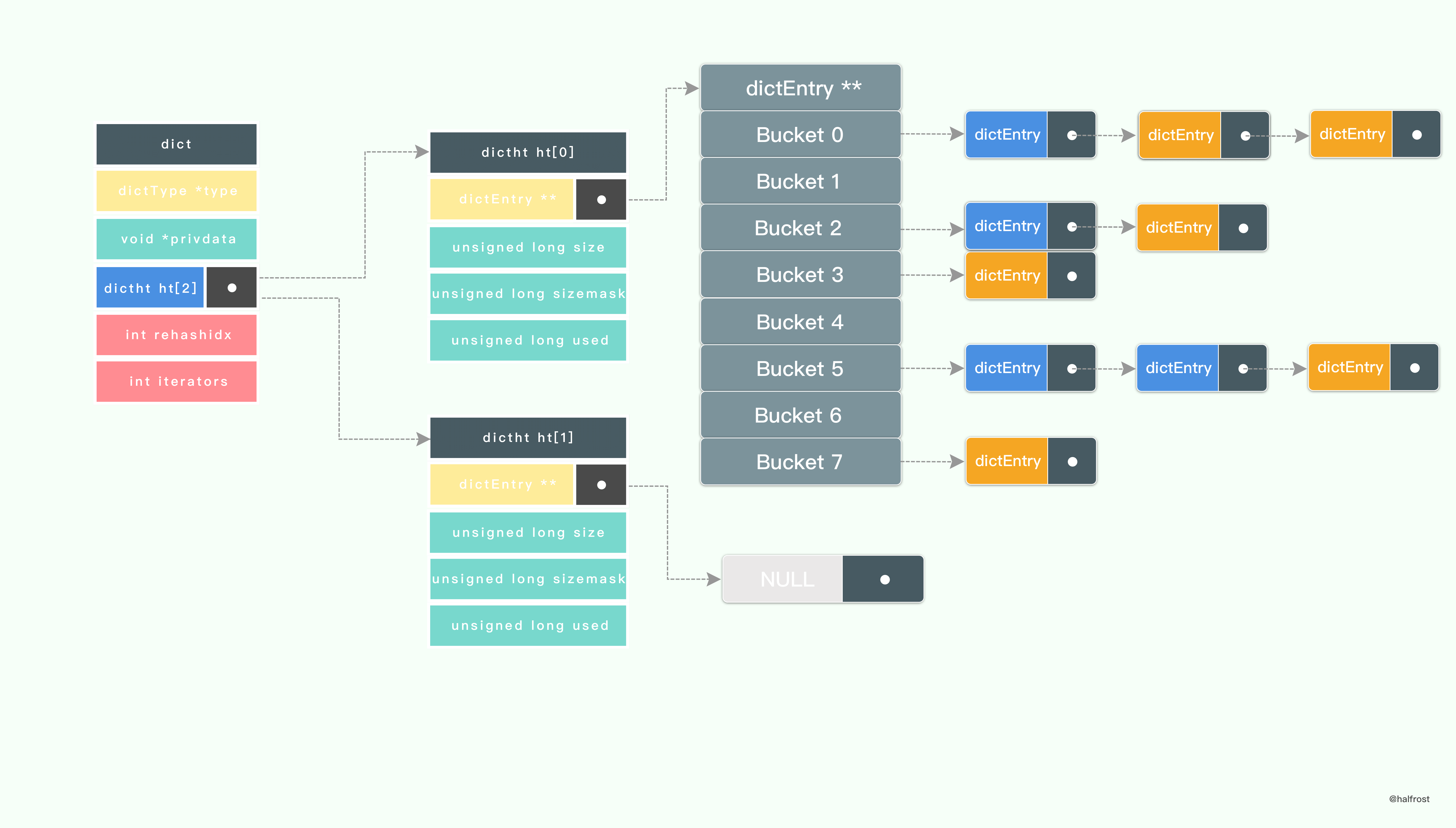
After rehashing finishes, the final state is shown above. If rehashing is needed again later, the same process is repeated. This multi-step, incremental rehashing approach is one of the reasons behind Redis’s high performance.
It is worth mentioning that Redis supports shrinking dictionaries as well. The procedure is simply the reverse of rehashing.
II. Red-Black Tree Optimization
At this point, readers should understand what approach can be used to control a map so that the probability of hash collisions remains low while the hash bucket array uses less space: choose a good hash algorithm and add an expansion mechanism.
Java further optimized the underlying implementation of HashMap in JDK 1.8.
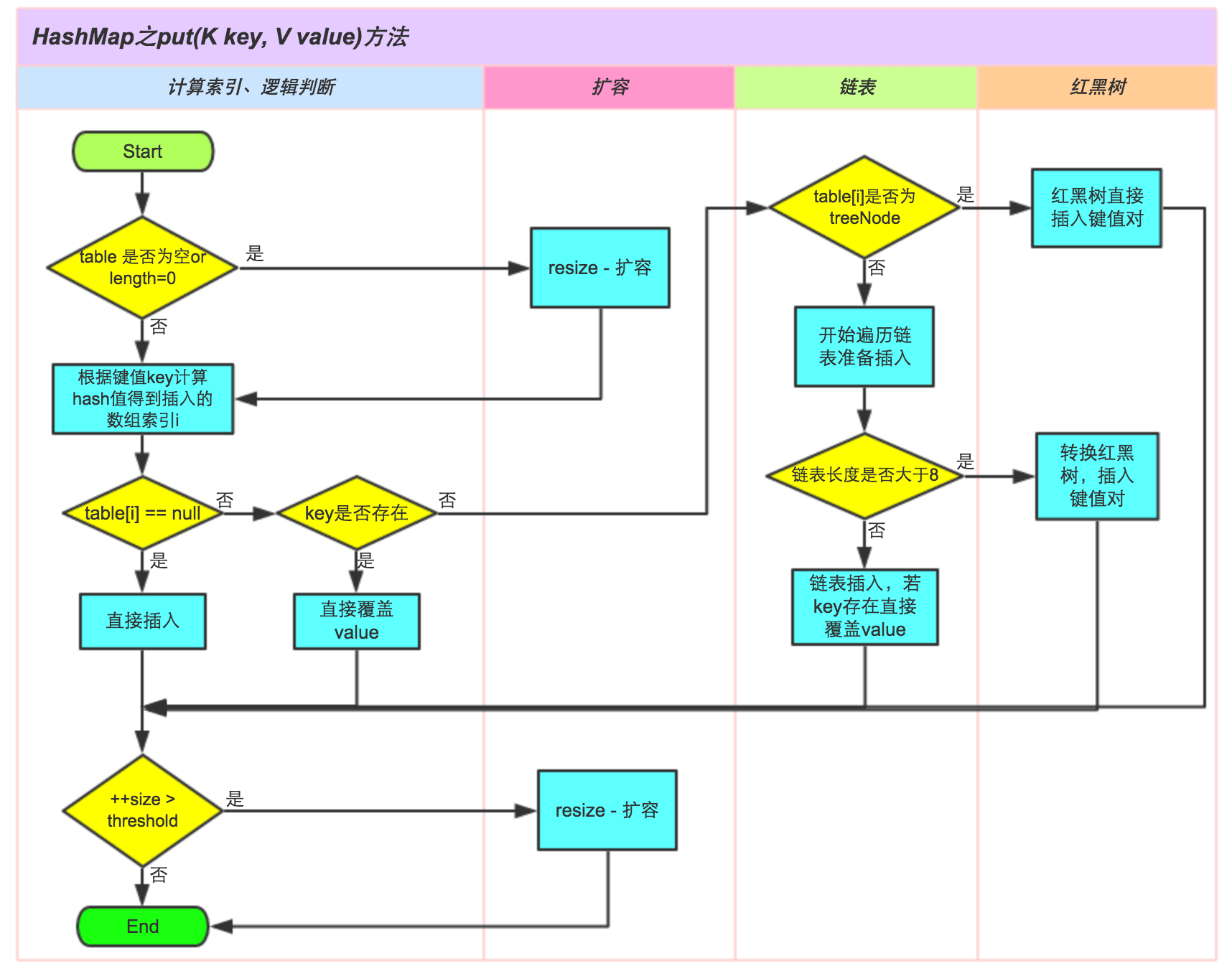
The diagram above is summarized from the Meituan Tech Blog. From it, we can see the following:
Java’s underlying initial bucket count is 16, and the default load factor is 0.75. That means resizing is triggered when the number of key-value pairs first reaches 12. The resize threshold is 64. After the bucket count exceeds 64, if the number of colliding nodes reaches 8 or more, conversion to a red-black tree is triggered. To prevent the underlying linked list from becoming too long, the list is converted into a red-black tree.
In other words, when the total number of buckets has not yet reached 64, even if the linked list length is 8, conversion to a red-black tree will not occur.
If the number of nodes drops below 6, the red-black tree degenerates back into a linked list.
Of course, the reason a red-black tree is used for optimization here is to ensure the worst case does not degrade to O(n). A red-black tree can guarantee a worst-case time complexity of O(log n).
The Meituan Tech Blog also mentions another optimization in Java JDK 1.8 that is worth learning from. During key-value node migration in rehashing, Java does not need to compute the hash again!
Because expansion uses powers of two (meaning the length is doubled), an element’s position is either unchanged or moved by a power-of-two offset from its original position. The diagram below illustrates this idea. n is the length of the table. Figure (a) shows examples of how key1 and key2 determine their index positions before expansion, while Figure (b) shows examples of how key1 and key2 determine their index positions after expansion. Here, hash1 is the result of applying the hash and high-bit operation for key1.
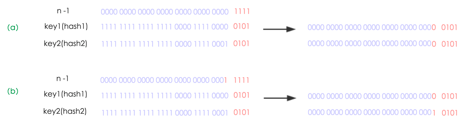
After recomputing the hash, because n becomes twice as large, the mask range of n-1 gains one extra bit in the high position (shown in red). Therefore, the new index changes as follows:

So after expansion, you only need to check whether the value of that bit corresponding to the expanded capacity is 0 or 1. If it is 0, the index remains unchanged. If it is 1, the new index is equal to the original index plus oldCap. This avoids computing the hash again.
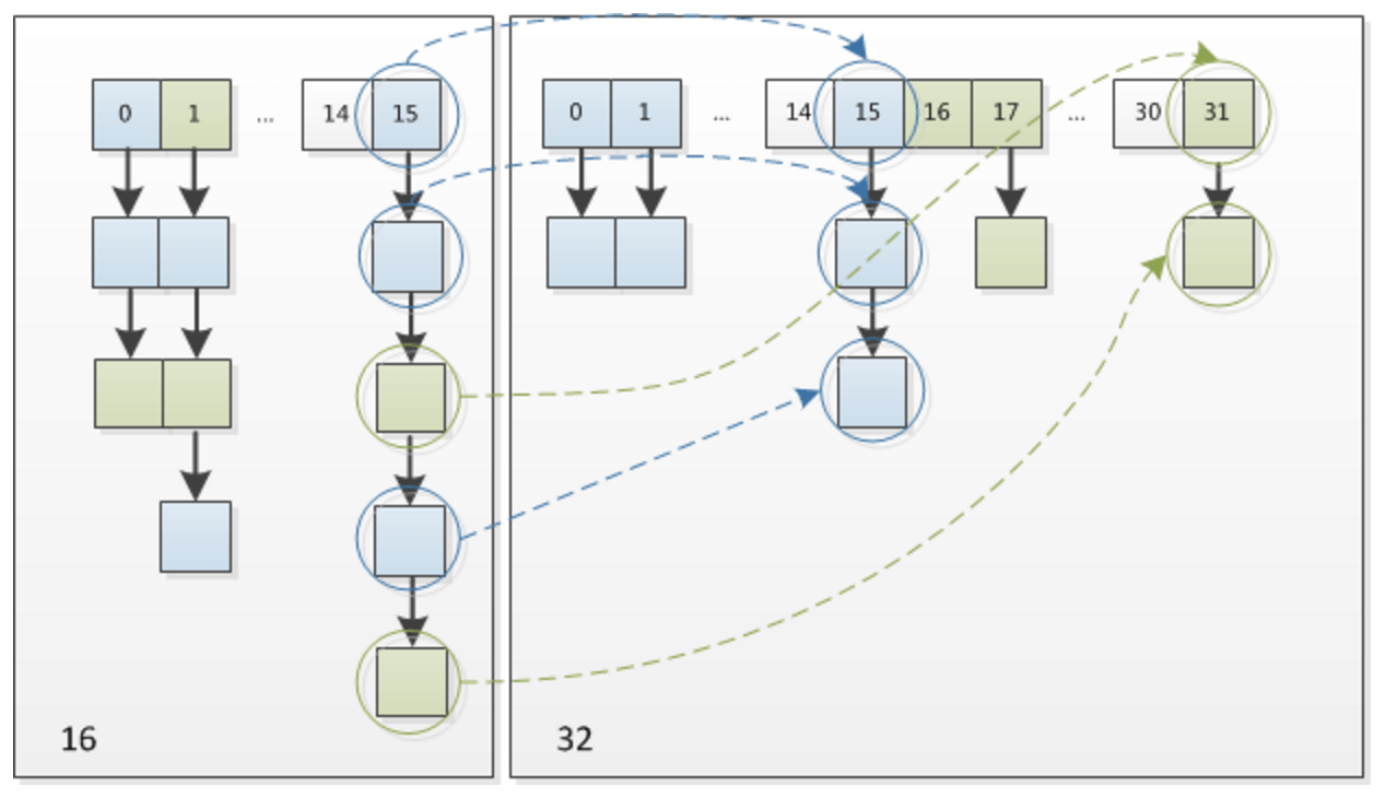
The diagram above shows the case of expanding from 16 to 32.
III. A Concrete Example of Go’s Map Implementation
At this point, readers should have some ideas of their own about how to design a map. You should now understand choosing a good hash algorithm, using a linked list + array as the underlying data structure, and how to expand and optimize it. You may think this article is already more than halfway done, but everything so far has been mostly theoretical. Next comes what may be the main focus of this article — analyzing a complete map implementation from scratch.
Next, I will analyze the underlying implementation of Go’s map. This also serves as a concrete example of a map implementation and several important operations: adding key-value pairs, deleting key-value pairs, and the expansion strategy.
Go’s map implementation is in /src/runtime/hashmap.go.
At the bottom, a map is essentially still a hash table.
First, let’s look at some constants defined by Go.
const (
	// Maximum number of key-value pairs a bucket can hold: 8 pairs.
	bucketCntBits = 3
	bucketCnt     = 1 << bucketCntBits

	// Threshold of the maximum load factor that triggers growth.
	loadFactor = 6.5

	// To keep things inline, the maximum key and value sizes are both 128 bytes; if exceeded, store a pointer instead.
	maxKeySize   = 128
	maxValueSize = 128

	// The data offset should be a multiple of bmap, but must be properly aligned.
	dataOffset = unsafe.Offsetof(struct {
		b bmap
		v int64
	}{}.v)

	// Some tophash values.
	empty          = 0 // No key-value pair.
	evacuatedEmpty = 1 // No key-value pair, and the bucket's key-values have been evacuated.
	evacuatedX     = 2 // Key-value pair is valid and has been evacuated to the first half of the table.
	evacuatedY     = 3 // Key-value pair is valid and has been evacuated to the second half of the table.
	minTopHash     = 4 // Minimum tophash.

	// Flags.
	iterator     = 1 // Iterator for current buckets.
	oldIterator  = 2 // Iterator for old buckets.
	hashWriting  = 4 // A goroutine is writing to the map.
	sameSizeGrow = 8 // The current map is growing to a new map of the same size.

	// Sentinel for the iterator to check bucket ID.
	noCheck = 1<<(8*sys.PtrSize) - 1
)
One point worth explaining here is how the threshold value 6.5 that triggers map growth is derived. If this value is too large, there will be too many overflow buckets, reducing lookup efficiency; if it is too small, storage space will be wasted.
According to Google developers, this value was chosen empirically based on measurements from a test program.
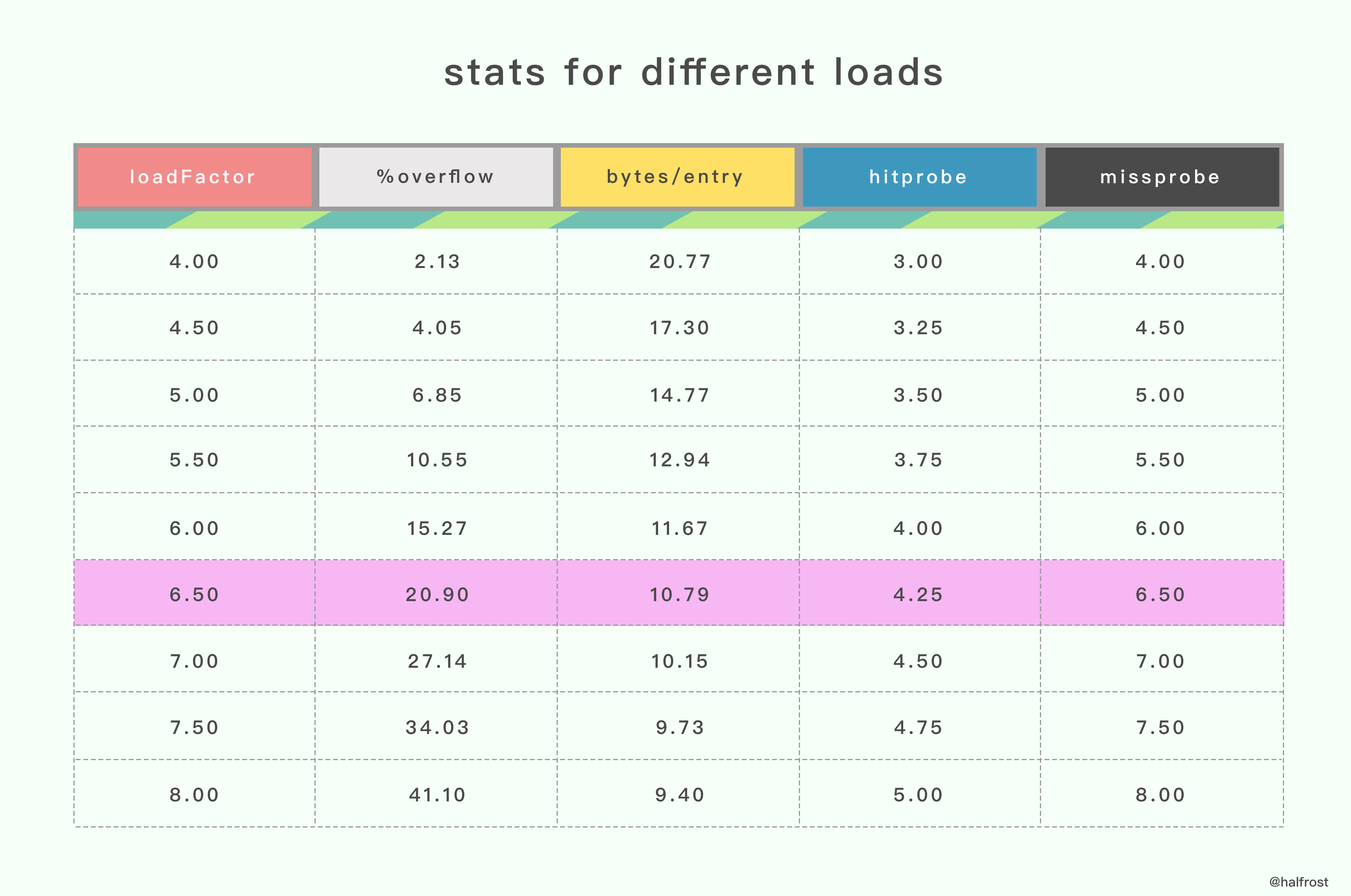
%overflow: Overflow rate: the average number of key-value pairs in a bucket at which it overflows.
bytes/entry: The average number of extra bytes required to store one key-value pair.
hitprobe: The average number of probes required to look up an existing key.
missprobe: The average number of probes required to look up a non-existent key.
Based on these sets of test data, 6.5 was ultimately chosen as the threshold load factor.
Next, let’s look at the definition of the map header in Go:
type hmap struct {
	count     int // length of the map
	flags     uint8
	B         uint8  // log base 2 of the number of buckets (can store about 6.5 * 2^B elements total)
	noverflow uint16 // approximate number of overflow buckets
	hash0     uint32 // hash seed

	buckets    unsafe.Pointer // array of 2^B buckets. nil when count==0.
	oldbuckets unsafe.Pointer // half the elements of the old bucket array
	nevacuate  uintptr        // counter during growth

	extra *mapextra // optional field
}
In Go’s map header structure, there are also two pointers to bucket arrays: buckets points to the new bucket array, and oldbuckets points to the old bucket array. This is similar to Redis dictionaries, which also have two dictht arrays.
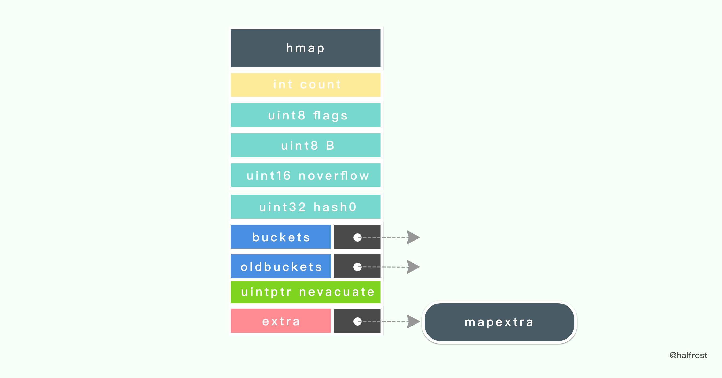
The last field of hmap is a pointer to a mapextra structure, defined as follows:
type mapextra struct {
	overflow [2]*[]*bmap
	nextOverflow *bmap
}
If a key-value pair cannot find a corresponding pointer, it is first stored in an overflow bucket, overflow. In mapextra, there is also a pointer to the next available overflow bucket.
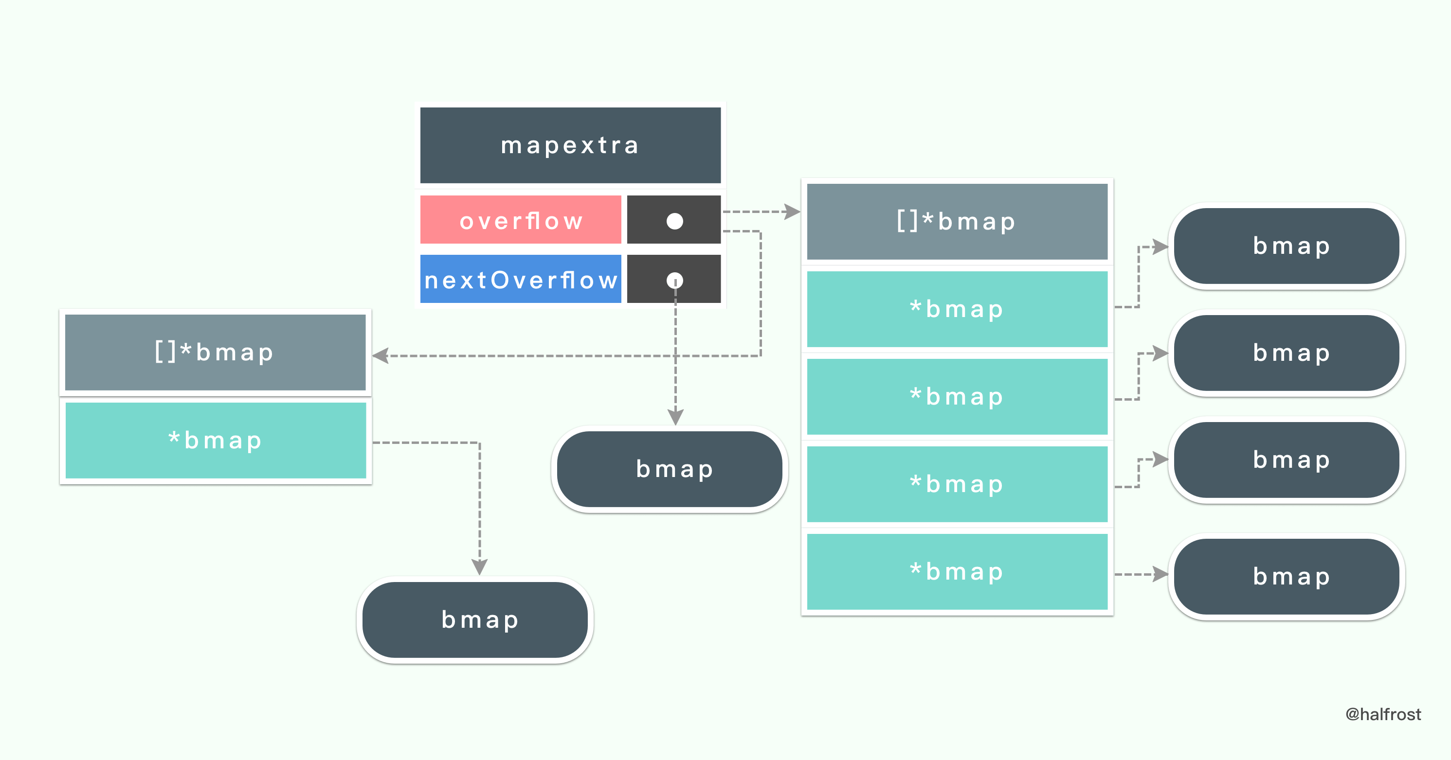
The overflow bucket overflow is an array containing two pointers to *bmap arrays. overflow[0] holds hmap.buckets. overflow[1] holds hmap.oldbuckets.
Now let’s look at the definition of the bucket data structure. bmap is the struct type corresponding to a bucket in Go’s map.
type bmap struct {
	tophash [bucketCnt]uint8
}
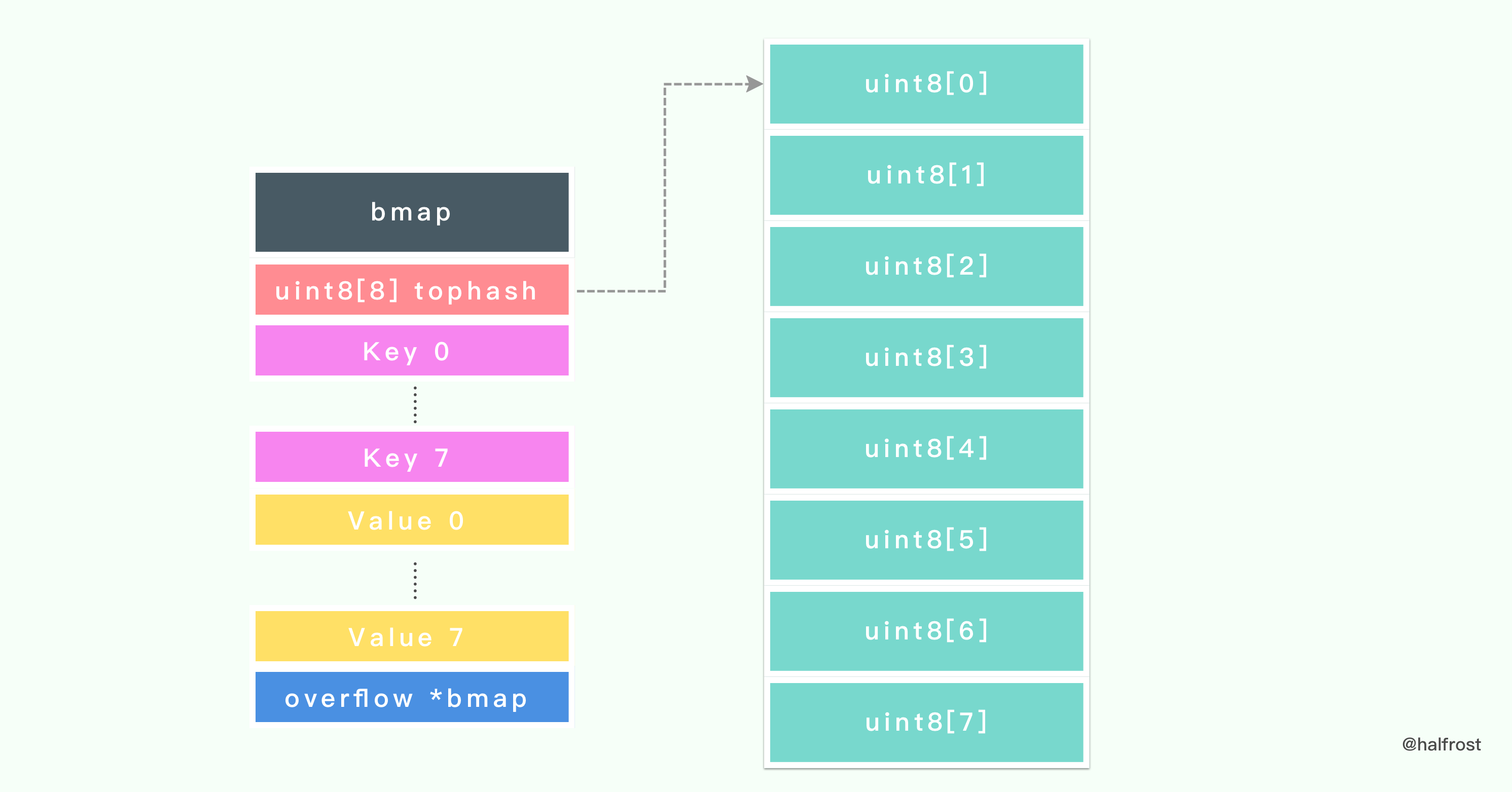
The definition of a bucket is fairly simple: it contains only an array of type uint8 with 8 elements. These 8 elements store the high 8 bits of the hash value.
After tophash, there are two additional regions in the memory layout. Immediately after tophash are 8 key-value pairs. They are arranged as 8 keys followed by 8 values.
After the 8 key-value pairs comes an overflow pointer, which points to the next bmap. From this, we can also see that Go handles hash collisions in map using a linked-list approach.
Why doesn’t Go store key-value pairs in the ordinary key/value, key/value, key/value… layout? Instead, it stores all the keys together, followed immediately by all the values. Why is it designed this way?
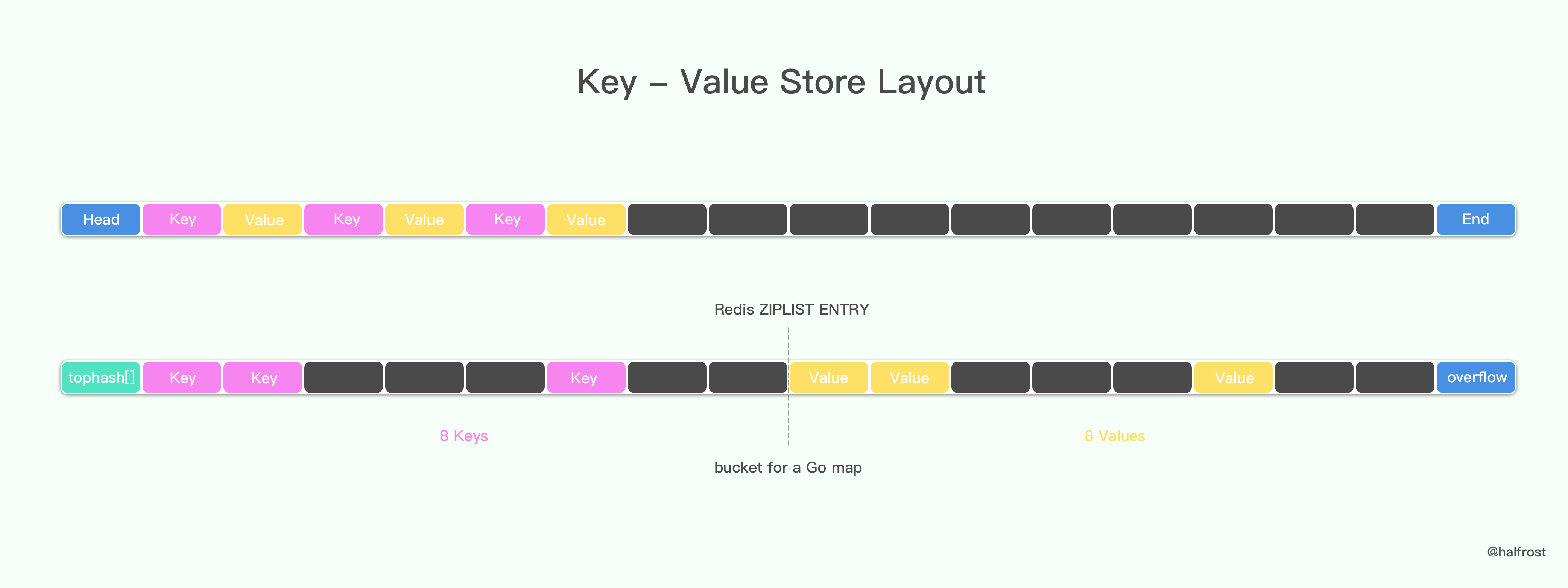
In Redis, when a hash table is encoded with REDIS\_ENCODING\_ZIPLIST, the program pushes keys and values together into the ziplist, thereby forming the key-value pair structure required to store the hash table, as shown above. Newly added key-value pairs are appended to the tail of the ziplist.
This structure has a drawback: if the stored keys and values have different types and occupy different numbers of bytes in memory, alignment is required. For example, consider storing a dictionary of type map[int64]int8.
To reduce the memory overhead caused by alignment, Go designs it as shown above.
If a map stores trillions of pieces of data, the memory saved here can be quite substantial.
1. Creating a Map
makemap creates a new Map. If the input parameter h is not nil, then the hmap of the map is this input hmap; if the input parameter bucket is not nil, then this bucket is used as the first bucket.
func makemap(t *maptype, hint int64, h *hmap, bucket unsafe.Pointer) *hmap {
	// hmap size is invalid
	if sz := unsafe.Sizeof(hmap{}); sz > 48 || sz != t.hmap.size {
		println("runtime: sizeof(hmap) =", sz, ", t.hmap.size =", t.hmap.size)
		throw("bad hmap size")
	}

	// Out-of-range hint values are set to 0
	if hint < 0 || hint > int64(maxSliceCap(t.bucket.size)) {
		hint = 0
	}

	// The key type is not supported by Go
	if !ismapkey(t.key) {
		throw("runtime.makemap: unsupported map key type")
	}

	// Check via the compiler and reflection whether the key size is valid
	if t.key.size > maxKeySize && (!t.indirectkey || t.keysize != uint8(sys.PtrSize)) ||
		t.key.size <= maxKeySize && (t.indirectkey || t.keysize != uint8(t.key.size)) {
		throw("key size wrong")
	}
	// Check via the compiler and reflection whether the value size is valid
	if t.elem.size > maxValueSize && (!t.indirectvalue || t.valuesize != uint8(sys.PtrSize)) ||
		t.elem.size <= maxValueSize && (t.indirectvalue || t.valuesize != uint8(t.elem.size)) {
		throw("value size wrong")
	}

	// Although we don't rely on the following variables, and the validity of these values can be checked at compile time,
	// we still check them here.

	// Key alignment exceeds the bucket count
	if t.key.align > bucketCnt {
		throw("key align too big")
	}
	// Value alignment exceeds the bucket count
	if t.elem.align > bucketCnt {
		throw("value align too big")
	}
	// Key size is not a multiple of key alignment
	if t.key.size%uintptr(t.key.align) != 0 {
		throw("key size not a multiple of key align")
	}
	// Value size is not a multiple of value alignment
	if t.elem.size%uintptr(t.elem.align) != 0 {
		throw("value size not a multiple of value align")
	}
	// Bucket count is too small for proper alignment
	if bucketCnt < 8 {
		throw("bucketsize too small for proper alignment")
	}
	// Data offset is not a multiple of key alignment, so key padding is needed in the bucket
	if dataOffset%uintptr(t.key.align) != 0 {
		throw("need padding in bucket (key)")
	}
	// Data offset is not a multiple of value alignment, so value padding is needed in the bucket
	if dataOffset%uintptr(t.elem.align) != 0 {
		throw("need padding in bucket (value)")
	}

	B := uint8(0)
	for ; overLoadFactor(hint, B); B++ {
	}

	// Allocate memory and initialize the hash table
	// If B = 0 at this point, the buckets field in hmap is allocated later
	// If hint is large, initializing this memory takes some time.
	buckets := bucket
	var extra *mapextra
	if B != 0 {
		var nextOverflow *bmap
		// Initialize bucket and nextOverflow
		buckets, nextOverflow = makeBucketArray(t, B)
		if nextOverflow != nil {
			extra = new(mapextra)
			extra.nextOverflow = nextOverflow
		}
	}

	// Initialize hmap
	if h == nil {
		h = (*hmap)(newobject(t.hmap))
	}
	h.count = 0
	h.B = B
	h.extra = extra
	h.flags = 0
	h.hash0 = fastrand()
	h.buckets = buckets
	h.oldbuckets = nil
	h.nevacuate = 0
	h.noverflow = 0

	return h
}
The most important part of creating a new map is allocating memory and initializing the hash table. When B is non-zero, mapextra is also initialized, and buckets are regenerated.
func makeBucketArray(t *maptype, b uint8) (buckets unsafe.Pointer, nextOverflow *bmap) {
	base := uintptr(1 << b)
	nbuckets := base
	if b >= 4 {
		nbuckets += 1 << (b - 4)
		sz := t.bucket.size * nbuckets
		up := roundupsize(sz)
		// If requesting buckets of size sz, the system can only return memory of size up, so the number of buckets is up / t.bucket.size
		if up != sz {
			nbuckets = up / t.bucket.size
		}
	}
	buckets = newarray(t.bucket, int(nbuckets))
	// When b > 4 and the computed number of buckets is not equal to 1 << b,
	if base != nbuckets {
		// At this point nbuckets is larger than base, so nbuckets - base nextOverflow buckets are preallocated
		nextOverflow = (*bmap)(add(buckets, base*uintptr(t.bucketsize)))
		last := (*bmap)(add(buckets, (nbuckets-1)*uintptr(t.bucketsize)))
		last.setoverflow(t, (*bmap)(buckets))
	}
	return buckets, nextOverflow
}
Here, newarray is already mallocgc.
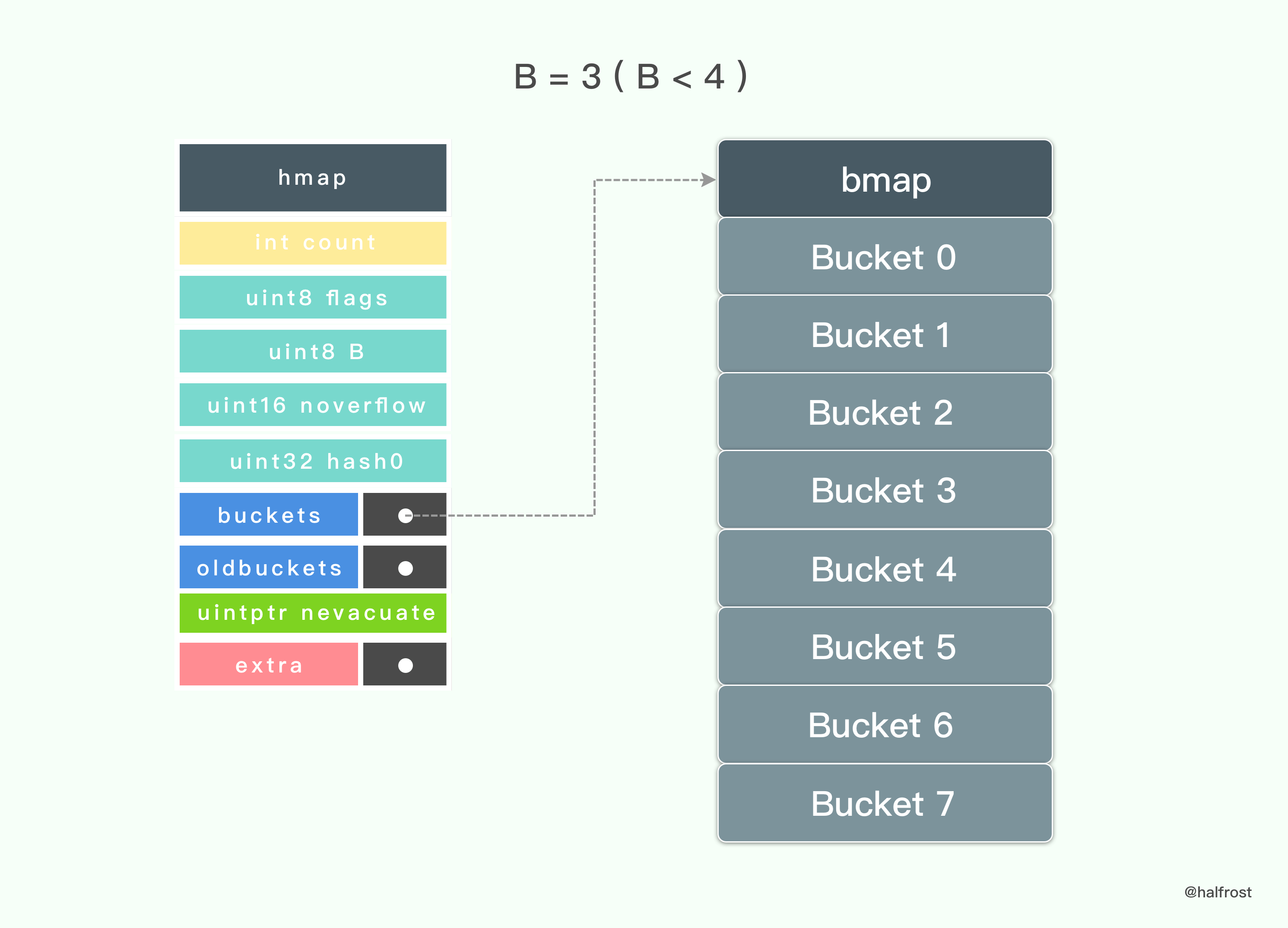
From the code above, we can see that only when B >= 4 will makeBucketArray create the nextOverflow pointer pointing to a bmap, and therefore mapextra will be created when the map creates its hmap.
When B = 3 (B < 4), initializing the hmap creates only 8 buckets.
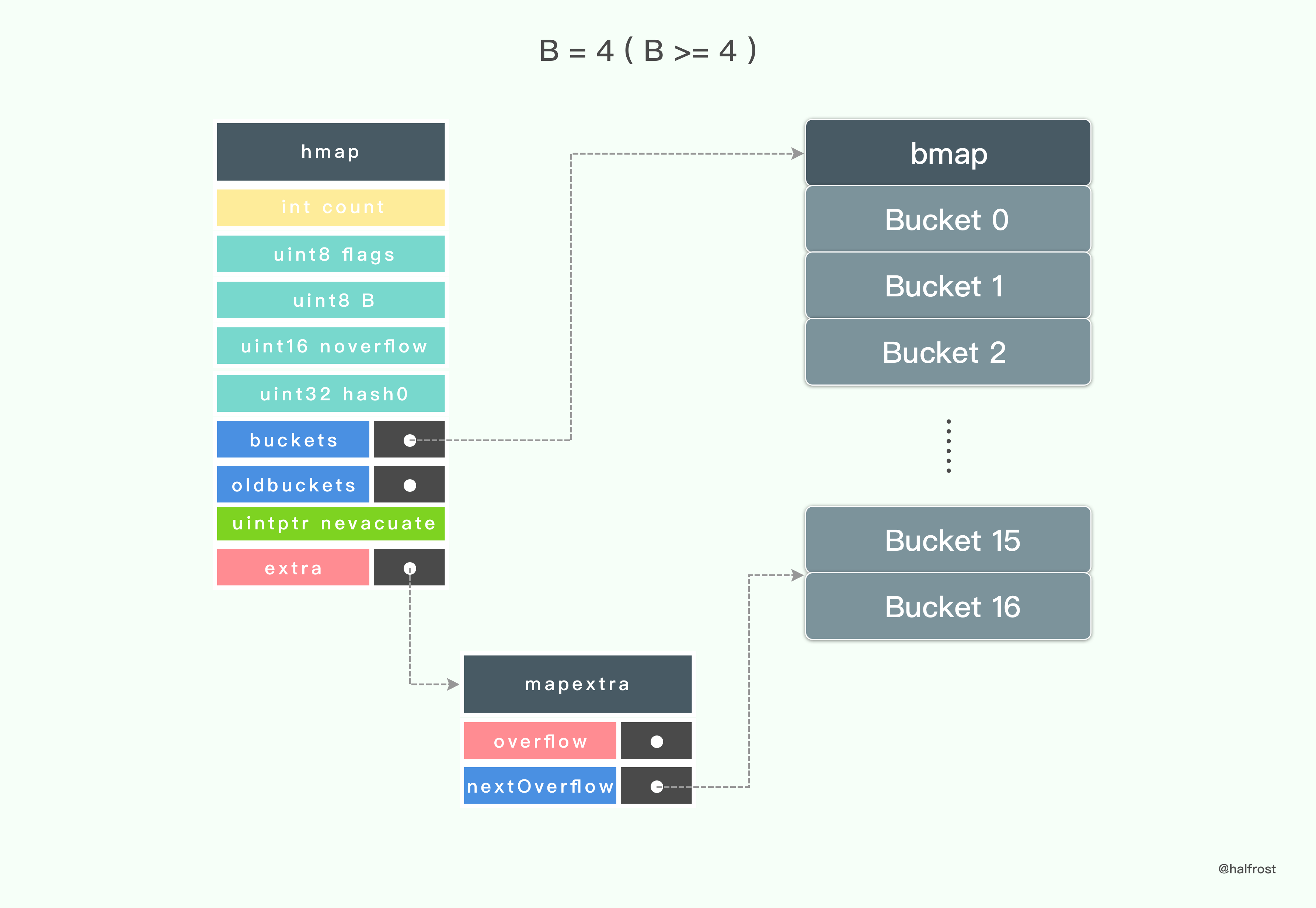
When B = 4 (B >= 4), initializing the hmap also creates an additional mapextra and initializes nextOverflow. The nextOverflow pointer in mapextra points to the end of the 16th bucket, i.e. the start address of the 17th bucket. In the 17th bucket (counting from 0, that is, the bucket with index 16), a pointer is stored starting at the address bucketsize - sys.PtrSize. This pointer points to the start address of the current entire bucket. This pointer is the overflow pointer of bmap.
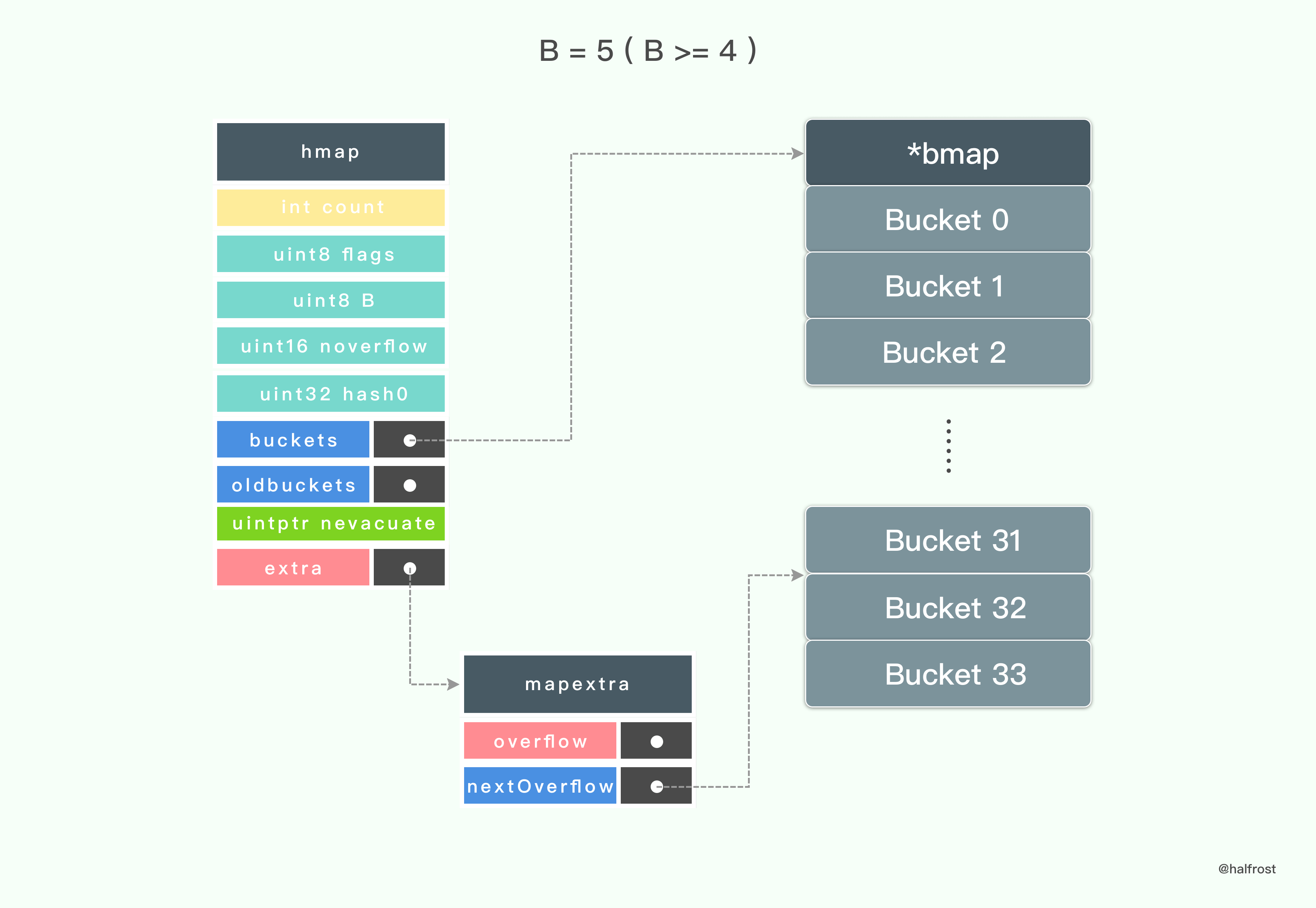
When B = 5 (B >= 4), initializing the hmap also creates an additional mapextra and initializes nextOverflow. At this point, a total of 34 buckets will be created. Similarly, an overflow pointer is stored starting at the address of the last bucket’s size minus the size of one pointer.
2. Looking Up a Key
In Go, when looking up a key that does not exist in a map, the lookup does not return nil; instead, it returns the zero value of the current type. For example, for a string it returns an empty string, and for an int it returns 0.
func mapaccess1(t *maptype, h *hmap, key unsafe.Pointer) unsafe.Pointer {
	if raceenabled && h != nil {
		// Get the caller's program counter
		callerpc := getcallerpc(unsafe.Pointer(&t))
		// Get mapaccess1's program counter
		pc := funcPC(mapaccess1)
		racereadpc(unsafe.Pointer(h), callerpc, pc)
		raceReadObjectPC(t.key, key, callerpc, pc)
	}
	if msanenabled && h != nil {
		msanread(key, t.key.size)
	}
	if h == nil || h.count == 0 {
		return unsafe.Pointer(&zeroVal[0])
	}
	// If there are concurrent reads and writes, throw immediately
	// Concurrency check: Go hashmap does not support concurrent access
	if h.flags&hashWriting != 0 {
		throw("concurrent map read and map write")
	}
	alg := t.key.alg
	// Compute the key's hash value
	hash := alg.hash(key, uintptr(h.hash0))
	m := uintptr(1)<<h.B - 1
	// Use hash % (1<<B - 1) to determine which bucket the key is in
	b := (*bmap)(add(h.buckets, (hash&m)*uintptr(t.bucketsize)))
	// If oldbuckets still exists
	if c := h.oldbuckets; c != nil {
		// Current growth is not same-size growth
		if !h.sameSizeGrow() {
			// If oldbuckets has not finished evacuation, look for the corresponding bucket in oldbuckets (low B-1 bits)
			// Otherwise, use the bucket in buckets (low B bits)
			// Halve the mask
			m >>= 1
		}

		oldb := (*bmap)(add(c, (hash&m)*uintptr(t.bucketsize)))
		if !evacuated(oldb) {
			// If the oldbuckets bucket exists and hasn't been evacuated, look for the key in the old bucket
			b = oldb
		}
	}
	// Extract the high 8 bits of the hash value
	top := uint8(hash >> (sys.PtrSize*8 - 8))
	// If top is less than minTopHash, add the minTopHash offset to it.
	// Because values in the range 0 to minTopHash are already used as marker values
	if top < minTopHash {
		top += minTopHash
	}
	for {
		for i := uintptr(0); i < bucketCnt; i++ {
			// If the high 8 bits of the hash don't match those recorded for the current key, check the next one
			// This comparison is efficient because it only compares the high 8 bits, not the entire hash value
			// If the high 8 bits differ, the hash values definitely differ; if they match, compare the full hash value
			if b.tophash[i] != top {
				continue
			}
			// The key is obtained by offset: bmap base address + offset of i key sizes
			k := add(unsafe.Pointer(b), dataOffset+i*uintptr(t.keysize))
			if t.indirectkey {
				k = *((*unsafe.Pointer)(k))
			}
			// Compare whether the key values are equal
			if alg.equal(key, k) {
				// If the key is found, extract the value
				// The value is obtained by offset: bmap base address + offset of 8 key sizes + offset of i value sizes
				v := add(unsafe.Pointer(b), dataOffset+bucketCnt*uintptr(t.keysize)+i*uintptr(t.valuesize))
				if t.indirectvalue {
					v = *((*unsafe.Pointer)(v))
				}
				return v
			}
		}
		// If the corresponding key is not found in the current bucket, look in the next bucket
		b = b.overflow(t)
		// If b == nil, all buckets have been searched; return the zero value for the corresponding type
		if b == nil {
			return unsafe.Pointer(&zeroVal[0])
		}
	}
}
The concrete implementation code is shown above; see the code for the detailed explanation.
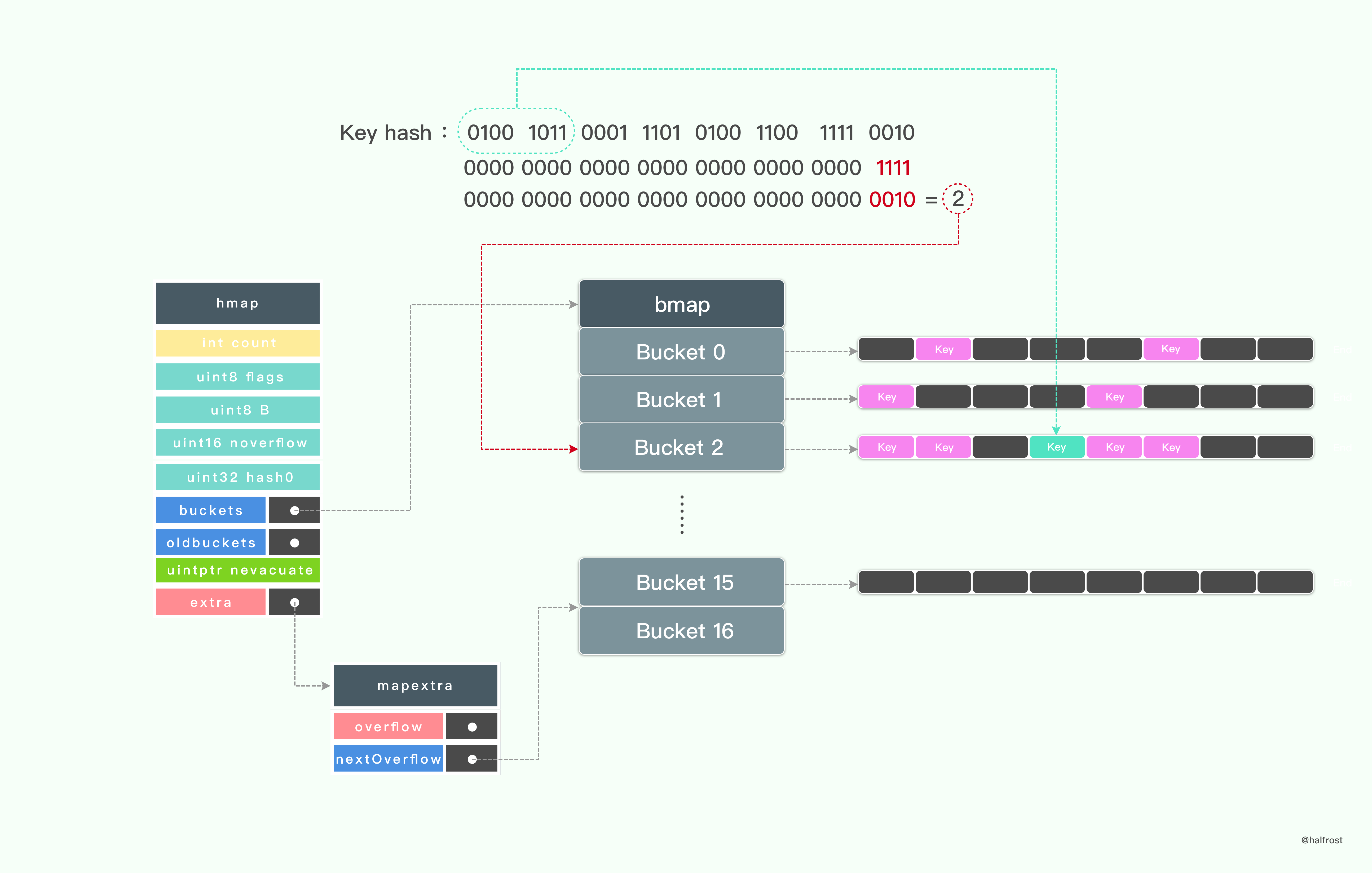
As shown in the figure above, this is the entire process of looking up a key.
First, compute the hash value for the key, then take the hash value modulo B.
There is an optimization opportunity here. For the computation m % n, if n is a multiple of 2, this modulo operation can be eliminated.
m % n = m & ( n - 1 )
This optimization avoids the costly modulo operation. In the example here, the computed value extracted is 0010, which is 2, so it corresponds to the 3rd bucket in the bucket array. Why the 3rd bucket? The base address points to bucket 0; offsetting downward by the size of 2 buckets moves to the base address of the 3rd bucket. For the concrete implementation, see the code above.
The lower B bits of the hash determine which bucket in the bucket array is used, while the upper 8 bits of the hash determine which position in the tophash array of this bucket array’s bmap may contain the key. As shown in the figure above, the upper 8 bits of the hash are compared against each value in the tophash array. If the upper 8 bits are not equal to tophash[i], the next entry is checked directly. If they are equal, the corresponding full key is retrieved from the bmap and compared again to see whether it matches exactly.
The entire lookup process first searches in oldbucket (if lodbucket exists), and then searches in the new bmap.
Some people may wonder why tophash is introduced here for an additional comparison.
tophash is introduced to speed up lookups. Because it stores only the upper 8 bits of the hash value, it is much faster than checking the full 64-bit value. By comparing the upper 8 bits, the index whose hash value has matching upper 8 bits can be found quickly. Then a full comparison is performed; if it still matches, the key is considered found.
If the key is found, the corresponding value is returned. If it is not found, the search continues in the overflow buckets until the last bucket is reached. If it still is not found, the zero value of the corresponding type is returned.
3. Inserting a Key
The process of inserting a key is largely the same as the process of looking up a key.
func mapassign(t *maptype, h *hmap, key unsafe.Pointer) unsafe.Pointer {
	if h == nil {
		panic(plainError("assignment to entry in nil map"))
	}
	if raceenabled {
		// Get the caller's program counter
		callerpc := getcallerpc(unsafe.Pointer(&t))
		// Get mapassign's program counter
		pc := funcPC(mapassign)
		racewritepc(unsafe.Pointer(h), callerpc, pc)
		raceReadObjectPC(t.key, key, callerpc, pc)
	}
	if msanenabled {
		msanread(key, t.key.size)
	}
	// If multiple threads read and write, throw immediately
	// Concurrency check: Go hashmap does not support concurrent access
	if h.flags&hashWriting != 0 {
		throw("concurrent map writes")
	}
	alg := t.key.alg
	// Compute the key's hash
	hash := alg.hash(key, uintptr(h.hash0))

	// Set hashWriting immediately after computing the hash; if writing is not fully done during hash computation, it may panic
	h.flags |= hashWriting

	// If the hmap has zero buckets, create one
	if h.buckets == nil {
		h.buckets = newarray(t.bucket, 1)
	}

again:
    // Take the hash modulo B to find the bucket
	bucket := hash & (uintptr(1)<<h.B - 1)
	// If still growing, continue growing
	if h.growing() {
		growWork(t, h, bucket)
	}
	// Use the low B bits of the hash to find the bucket
	b := (*bmap)(unsafe.Pointer(uintptr(h.buckets) + bucket*uintptr(t.bucketsize)))
	// Compute the high 8 bits of the hash
	top := uint8(hash >> (sys.PtrSize*8 - 8))
	if top < minTopHash {
		top += minTopHash
	}

	var inserti *uint8
	var insertk unsafe.Pointer
	var val unsafe.Pointer
	for {
		// Iterate all key-value pairs in the current bucket to find the value for key
		for i := uintptr(0); i < bucketCnt; i++ {
			if b.tophash[i] != top {
				if b.tophash[i] == empty && inserti == nil {
					// If not found later, first record this spot for insertion
					inserti = &b.tophash[i]
					// Compute the position offset by i keys
					insertk = add(unsafe.Pointer(b), dataOffset+i*uintptr(t.keysize))
					// Compute val's position: bucket start + size of 8 keys + size of i values
					val = add(unsafe.Pointer(b), dataOffset+bucketCnt*uintptr(t.keysize)+i*uintptr(t.valuesize))
				}
				continue
			}
			// Get each key
			k := add(unsafe.Pointer(b), dataOffset+i*uintptr(t.keysize))
			// If the key is a pointer, get the key it points to
			if t.indirectkey {
				k = *((*unsafe.Pointer)(k))
			}
			// Compare whether the keys are equal
			if !alg.equal(key, k) {
				continue
			}
			// If an update is needed, copy t.key from k to key
			if t.needkeyupdate {
				typedmemmove(t.key, k, key)
			}
			// Compute val's position: bucket start + size of 8 keys + size of i values
			val = add(unsafe.Pointer(b), dataOffset+bucketCnt*uintptr(t.keysize)+i*uintptr(t.valuesize))
			goto done
		}
		ovf := b.overflow(t)
		if ovf == nil {
			break
		}
		b = ovf
	}

	// The current key was not found, and check the maximum load factor; if it reaches the maximum load factor, or there are many overflow buckets
	if !h.growing() && (overLoadFactor(int64(h.count), h.B) || tooManyOverflowBuckets(h.noverflow, h.B)) {
		// Start growing
		hashGrow(t, h)
		goto again // Growing the table invalidates everything, so try again
	}
	// If no empty slot can be found to insert the key
	if inserti == nil {
		// all current buckets are full, allocate a new one.
		// Means all current buckets are full, so create a new one
		newb := h.newoverflow(t, b)
		inserti = &newb.tophash[0]
		insertk = add(unsafe.Pointer(newb), dataOffset)
		val = add(insertk, bucketCnt*uintptr(t.keysize))
	}

	// store new key/value at insert position
	if t.indirectkey {
		// If storing a pointer to the key, use insertk to store the key's address
		kmem := newobject(t.key)
		*(*unsafe.Pointer)(insertk) = kmem
		insertk = kmem
	}
	if t.indirectvalue {
		// If storing a pointer to the value, use val to store the key's address
		vmem := newobject(t.elem)
		*(*unsafe.Pointer)(val) = vmem
	}
	// Copy t.key from insertk to the key position
	typedmemmove(t.key, insertk, key)
	*inserti = top
	// Total number of keys stored in hmap + 1
	h.count++

done:
	// Disallow concurrent writes
	if h.flags&hashWriting == 0 {
		throw("concurrent map writes")
	}
	h.flags &^= hashWriting
	if t.indirectvalue {
		// If value stores a pointer, get the value it points to
		val = *((*unsafe.Pointer)(val))
	}
	return val
}
When inserting a key, there are a few differences from looking up a key that are worth noting:
- If the key to be inserted is found, simply update the corresponding value directly.
- If the key to be inserted is not found in the bmap, there are several possible cases. Case 1: There is still an empty slot in the bmap. While traversing the bmap, pre-mark the empty slot. If the lookup finishes and the key still has not been found, place the key into the empty slot that was marked during traversal. Case 2: There are no empty slots left in the bmap. At this point, the bmap is very full. You need to check whether the maximum load factor has been reached. If it has, grow the map immediately. After growth, insert the key into the new bucket; the flow is the same as described above. If the maximum load factor has not been reached, create a new bmap and point the previous bmap’s overflow pointer to the new bmap.
- During growth, oldbucket is frozen. When looking up a key, the lookup will search oldbucket, but data will not be inserted into oldbucket. If the corresponding key is found in oldbucket, the approach is to migrate it to the new bmap and then add the evacuated marker.
The rest of the flow is basically the same as key lookup, so it will not be repeated here.
3. Deleting a Key
func mapdelete(t *maptype, h *hmap, key unsafe.Pointer) {
	if raceenabled && h != nil {
		// Get the caller's program counter
		callerpc := getcallerpc(unsafe.Pointer(&t))
		// Get mapdelete's program counter
		pc := funcPC(mapdelete)
		racewritepc(unsafe.Pointer(h), callerpc, pc)
		raceReadObjectPC(t.key, key, callerpc, pc)
	}
	if msanenabled && h != nil {
		msanread(key, t.key.size)
	}
	if h == nil || h.count == 0 {
		return
	}
	// If multiple threads read/write, throw immediately
	// Concurrency check: Go hashmap does not support concurrent access
	if h.flags&hashWriting != 0 {
		throw("concurrent map writes")
	}

	alg := t.key.alg
	// Compute the hash of the key
	hash := alg.hash(key, uintptr(h.hash0))

	// Set hashWriting immediately after computing the hash; if a write occurs during hash computation, it may panic
	h.flags |= hashWriting

	bucket := hash & (uintptr(1)<<h.B - 1)
	// If still growing, continue growing
	if h.growing() {
		growWork(t, h, bucket)
	}
	// Use the low B bits of the hash to find the bucket
	b := (*bmap)(unsafe.Pointer(uintptr(h.buckets) + bucket*uintptr(t.bucketsize)))
	// Compute the high 8 bits of the hash
	top := uint8(hash >> (sys.PtrSize*8 - 8))
	if top < minTopHash {
		top += minTopHash
	}
	for {
		// Iterate over all entries in the current bucket to find the value for key
		for i := uintptr(0); i < bucketCnt; i++ {
			if b.tophash[i] != top {
				continue
			}
			k := add(unsafe.Pointer(b), dataOffset+i*uintptr(t.keysize))
			// If k is a pointer to the key, retrieve the key value here
			k2 := k
			if t.indirectkey {
				k2 = *((*unsafe.Pointer)(k2))
			}
			if !alg.equal(key, k2) {
				continue
			}
			// Set the key pointer to nil
			if t.indirectkey {
				*(*unsafe.Pointer)(k) = nil
			} else {
			// Clear the key's memory
				typedmemclr(t.key, k)
			}
			v := unsafe.Pointer(uintptr(unsafe.Pointer(b)) + dataOffset + bucketCnt*uintptr(t.keysize) + i*uintptr(t.valuesize))
			// Set the value pointer to nil
			if t.indirectvalue {
				*(*unsafe.Pointer)(v) = nil
			} else {
			// Clear the value's memory
				typedmemclr(t.elem, v)
			}
			// Clear the value in tophash
			b.tophash[i] = empty
			// Decrement the total number of keys in the map by 1
			h.count--
			goto done
		}
		// If not found, continue searching overflow buckets until the last one
		b = b.overflow(t)
		if b == nil {
			goto done
		}
	}

done:
	if h.flags&hashWriting == 0 {
		throw("concurrent map writes")
	}
	h.flags &^= hashWriting
}
The main flow of deletion is roughly the same as the key lookup flow. After the corresponding key is found, if it is referenced by a pointer to the original key, set that pointer to nil. If it is a value, clear the memory where it resides. The value in tophash also needs to be cleared, and finally the map’s total key count is decremented by 1.
If deletion happens during growth, the delete operation will delete from the new bmap after growth.
The lookup process still traverses all the way to the last bmap bucket in the linked list.
4. Incremental Doubling Growth
This part is arguably one of the core parts of the entire Map implementation. We all know that as a Map keeps loading key values, lookup efficiency becomes lower and lower. If growth is not performed at this point, hash collisions will make the linked list longer and longer, and performance will degrade accordingly. Growth is inevitable.
However, if writes of key values are blocked during growth, processing large datasets can introduce a period of non-responsiveness. In a highly real-time system, each growth operation could cause the system to stall for several seconds, during which it cannot respond to any requests. This kind of performance is obviously unacceptable. Therefore, growth must be performed without affecting writes. This is where incremental growth comes in.
Incremental growth is already widely used in practice. Redis, mentioned earlier as an example, uses an incremental growth strategy.
Next, let’s look at how Go performs incremental growth.
When Go’s mapassign inserts a key value and mapdelete deletes a key value, they both check whether growth is currently in progress.
func growWork(t *maptype, h *hmap, bucket uintptr) {
	// Ensure we've evacuated all oldbuckets
	evacuate(t, h, bucket&h.oldbucketmask())

	// Evacuate one more marked bucket
	if h.growing() {
		evacuate(t, h, h.nevacuate)
	}
}
From this, we can see that each time growWork is executed, it migrates 2 buckets. One is the current bucket, which counts as local migration; the other is the bucket pointed to by nevacuate in hmap, which counts as incremental migration.
When inserting a Key value, if expansion is currently in progress, oldbucket is frozen. Lookups will first search oldbucket, but data will not be inserted into oldbucket. Only if the corresponding key is found in oldbucket will it be migrated to the new bucket and marked as evalucated.
When deleting a Key value, if expansion is currently in progress, the bucket—that is, the new bucket—is searched first. Once found, its corresponding Key and Value are both cleared. Only if it cannot be found in bucket will oldbucket be searched.
Each time a Key value is inserted, it checks whether the current load factor exceeds 6.5. If this limit has been reached, the expansion operation hashGrow is executed immediately. This is the preparation work before expansion.
func hashGrow(t *maptype, h *hmap) {
	// If the maximum load factor is reached, grow.
	// Otherwise, a bucket's linked list will be followed by many overflow buckets.
	bigger := uint8(1)
	if !overLoadFactor(int64(h.count), h.B) {
		bigger = 0
		h.flags |= sameSizeGrow
	}
	// Point hmap's old bucket pointer to the current buckets
	oldbuckets := h.buckets
	// Create the new grown buckets; hmap's buckets pointer points to them.
	newbuckets, nextOverflow := makeBucketArray(t, h.B+bigger)

	flags := h.flags &^ (iterator | oldIterator)
	if h.flags&iterator != 0 {
		flags |= oldIterator
	}
	// Increment B by the new value
	h.B += bigger
	h.flags = flags
	// Old bucket pointer points to the current buckets
	h.oldbuckets = oldbuckets
	// New bucket pointer points to the grown buckets
	h.buckets = newbuckets
	h.nevacuate = 0
	h.noverflow = 0

	if h.extra != nil && h.extra.overflow[0] != nil {
		if h.extra.overflow[1] != nil {
			throw("overflow is not nil")
		}
		// Swap the targets of overflow[0] and overflow[1]
		h.extra.overflow[1] = h.extra.overflow[0]
		h.extra.overflow[0] = nil
	}
	if nextOverflow != nil {
		if h.extra == nil {
			// Create mapextra
			h.extra = new(mapextra)
		}
		h.extra.nextOverflow = nextOverflow
	}

	// The actual key-value copying happens in evacuate()
}
Its flow can be illustrated as follows:
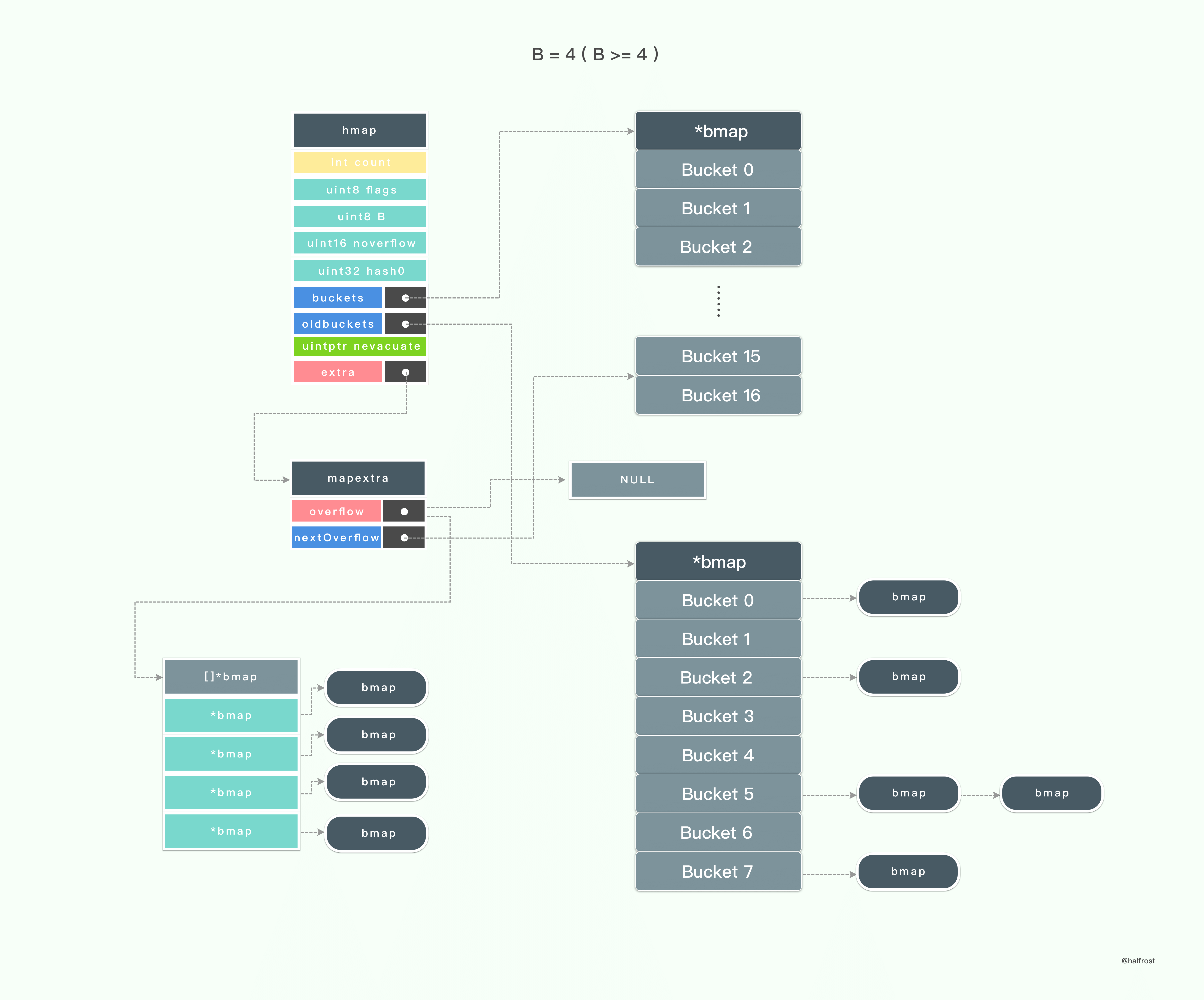
The hashGrow operation is the preparation before growing the map; the actual copying happens in evacuate.
hashGrow first creates the new bucket array after growth. The new bucket array is twice the size of the previous one. Then hmap’s buckets points to this newly grown bucket array, while oldbuckets points to the current bucket array.
After handling hmap, it handles mapextra: nextOverflow points to the original overflow pointer, and the overflow pointer is set to nil.
At this point, the preparation before growing is complete.
func evacuate(t *maptype, h *hmap, oldbucket uintptr) {
	b := (*bmap)(add(h.oldbuckets, oldbucket*uintptr(t.bucketsize)))
	// Number of buckets before growing
	newbit := h.noldbuckets()
	alg := t.key.alg
	if !evacuated(b) {
		// TODO: reuse overflow buckets instead of using new ones, if there
		// is no iterator using the old buckets.  (If !oldIterator.)

		var (
			x, y   *bmap          // Low and high buckets in the new buckets
			xi, yi int            // Indices for key and value are xi and yi respectively
			xk, yk unsafe.Pointer // Pointers to the key values of x and y
			xv, yv unsafe.Pointer // Pointers to the value values of x and y
		)
		// Low buckets in the new buckets
		x = (*bmap)(add(h.buckets, oldbucket*uintptr(t.bucketsize)))
		xi = 0
		// First key in the low bucket after growing
		xk = add(unsafe.Pointer(x), dataOffset)
		// Value corresponding to the first key in the low bucket after growing
		xv = add(xk, bucketCnt*uintptr(t.keysize))
		// If this is not a same-size grow
		if !h.sameSizeGrow() {
			y = (*bmap)(add(h.buckets, (oldbucket+newbit)*uintptr(t.bucketsize)))
			yi = 0
			yk = add(unsafe.Pointer(y), dataOffset)
			yv = add(yk, bucketCnt*uintptr(t.keysize))
		}
		// Iterate over overflow buckets in order
		for ; b != nil; b = b.overflow(t) {
			k := add(unsafe.Pointer(b), dataOffset)
			v := add(k, bucketCnt*uintptr(t.keysize))
			// Iterate over key-value pairs
			for i := 0; i < bucketCnt; i, k, v = i+1, add(k, uintptr(t.keysize)), add(v, uintptr(t.valuesize)) {
				top := b.tophash[i]
				if top == empty {
					b.tophash[i] = evacuatedEmpty
					continue
				}
				if top < minTopHash {
					throw("bad map state")
				}
				k2 := k
				// If the key is a pointer, get the value it points to
				if t.indirectkey {
					k2 = *((*unsafe.Pointer)(k2))
				}
				useX := true
				if !h.sameSizeGrow() {
					// If this is not a same-size grow, recalculate the hash value, whether in high bucket x or low bucket y
					hash := alg.hash(k2, uintptr(h.hash0))
					if h.flags&iterator != 0 {
						if !t.reflexivekey && !alg.equal(k2, k2) {
							// If two keys are not equal, their old hash values are very likely not equal either.
							// tophash is not very meaningful for keys being evacuated, so we use the low bit of tophash to help growing and mark states.
							// Recalculate some new random hash values for the next level, so these keys can still be evenly distributed across all buckets after multiple grows
							// Check whether the lowest bit of top is 1
							if top&1 != 0 {
								hash |= newbit
							} else {
								hash &^= newbit
							}
							top = uint8(hash >> (sys.PtrSize*8 - 8))
							if top < minTopHash {
								top += minTopHash
							}
						}
					}
					useX = hash&newbit == 0
				}
				if useX {
					// Mark that the low bucket exists in tophash
					b.tophash[i] = evacuatedX
					// If the key index reaches the end of the bucket, create a new overflow
					if xi == bucketCnt {
						newx := h.newoverflow(t, x)
						x = newx
						xi = 0
						xk = add(unsafe.Pointer(x), dataOffset)
						xv = add(xk, bucketCnt*uintptr(t.keysize))
					}
					// Store the high 8 bits of the hash in tophash again
					x.tophash[xi] = top
					if t.indirectkey {
						// If a pointer points to the key, copy the pointer
						*(*unsafe.Pointer)(xk) = k2 // copy pointer
					} else {
						// If a pointer points to the key, copy the value
						typedmemmove(t.key, xk, k) // copy value
					}
					// Copy the value similarly
					if t.indirectvalue {
						*(*unsafe.Pointer)(xv) = *(*unsafe.Pointer)(v)
					} else {
						typedmemmove(t.elem, xv, v)
					}
					// Continue migrating the next one
					xi++
					xk = add(xk, uintptr(t.keysize))
					xv = add(xv, uintptr(t.valuesize))
				} else {
					// This is high bucket y; migration is the same as the low bucket x above, so no further details below
					b.tophash[i] = evacuatedY
					if yi == bucketCnt {
						newy := h.newoverflow(t, y)
						y = newy
						yi = 0
						yk = add(unsafe.Pointer(y), dataOffset)
						yv = add(yk, bucketCnt*uintptr(t.keysize))
					}
					y.tophash[yi] = top
					if t.indirectkey {
						*(*unsafe.Pointer)(yk) = k2
					} else {
						typedmemmove(t.key, yk, k)
					}
					if t.indirectvalue {
						*(*unsafe.Pointer)(yv) = *(*unsafe.Pointer)(v)
					} else {
						typedmemmove(t.elem, yv, v)
					}
					yi++
					yk = add(yk, uintptr(t.keysize))
					yv = add(yv, uintptr(t.valuesize))
				}
			}
		}
		// Unlink the overflow buckets & clear key/value to help GC.
		if h.flags&oldIterator == 0 {
			b = (*bmap)(add(h.oldbuckets, oldbucket*uintptr(t.bucketsize)))
			// Preserve b.tophash because the evacuation
			// state is maintained there.
			if t.bucket.kind&kindNoPointers == 0 {
				memclrHasPointers(add(unsafe.Pointer(b), dataOffset), uintptr(t.bucketsize)-dataOffset)
			} else {
				memclrNoHeapPointers(add(unsafe.Pointer(b), dataOffset), uintptr(t.bucketsize)-dataOffset)
			}
		}
	}

	// Advance evacuation mark
	if oldbucket == h.nevacuate {
		h.nevacuate = oldbucket + 1
		// Experiments suggest that 1024 is overkill by at least an order of magnitude.
		// Put it in there as a safeguard anyway, to ensure O(1) behavior.
		stop := h.nevacuate + 1024
		if stop > newbit {
			stop = newbit
		}
		for h.nevacuate != stop && bucketEvacuated(t, h, h.nevacuate) {
			h.nevacuate++
		}
		if h.nevacuate == newbit { // newbit == # of oldbuckets
			// Growing is all done. Free old main bucket array.
			h.oldbuckets = nil
			// Can discard old overflow buckets as well.
			// If they are still referenced by an iterator,
			// then the iterator holds a pointers to the slice.
			if h.extra != nil {
				h.extra.overflow[1] = nil
			}
			h.flags &^= sameSizeGrow
		}
	}
}
The function above performs the core copy work in the migration process.
The overall migration process is not difficult. What needs clarification here is the meaning of x and y. After growth, the new bucket array is twice the size of the original bucket array. x represents the lower half of the new bucket array, and y represents the upper half. The other variables are just markers—cursors and markers for the original positions of key-value pairs. See the code comments for details.
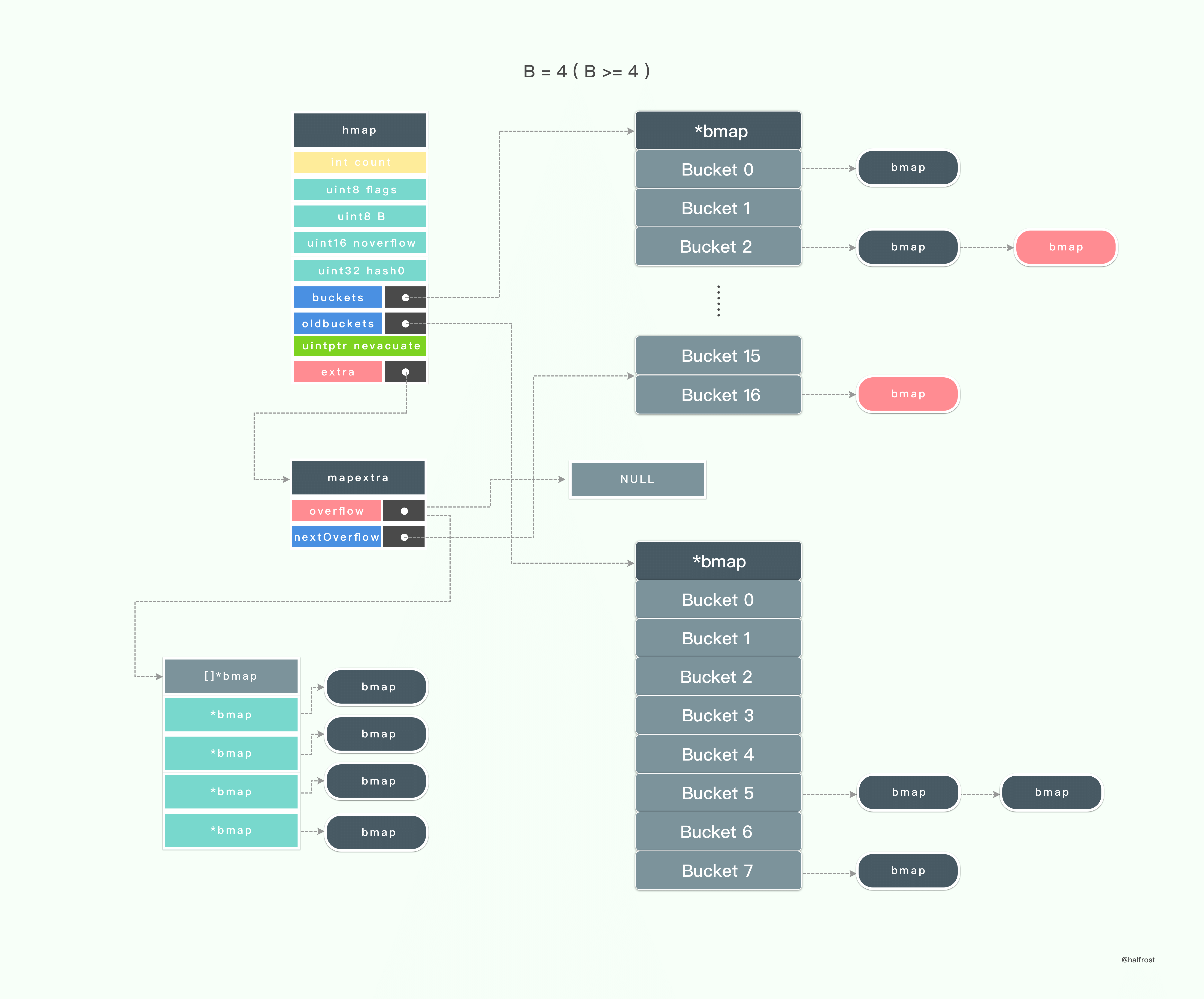
The figure above shows the process after migration starts. You can see that buckets in the old bucket array are being migrated to the new buckets, while new key values are also continuously being written into the new buckets.
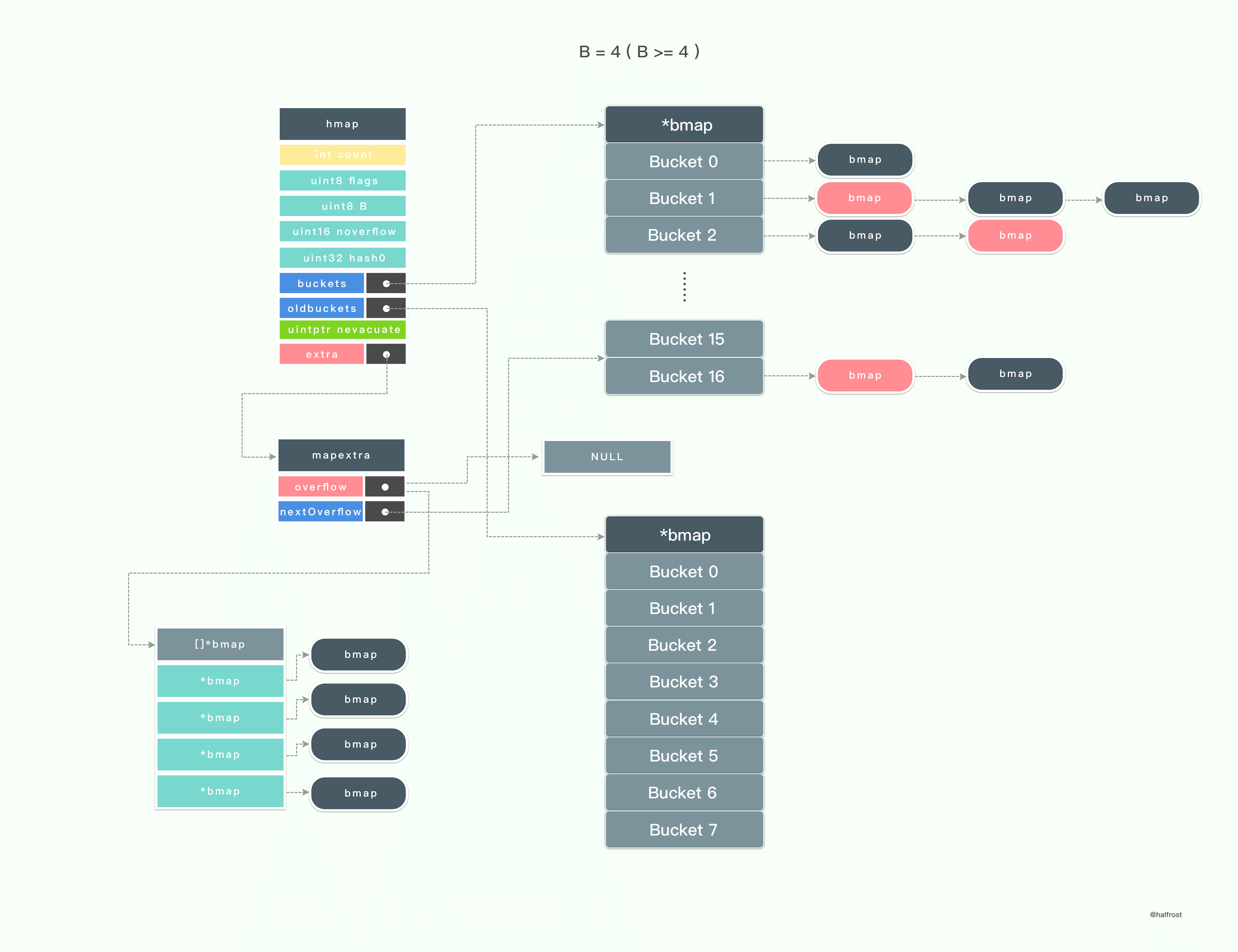
Key-value pairs continue to be copied until all key-value pairs in the old buckets have been copied into the new buckets.
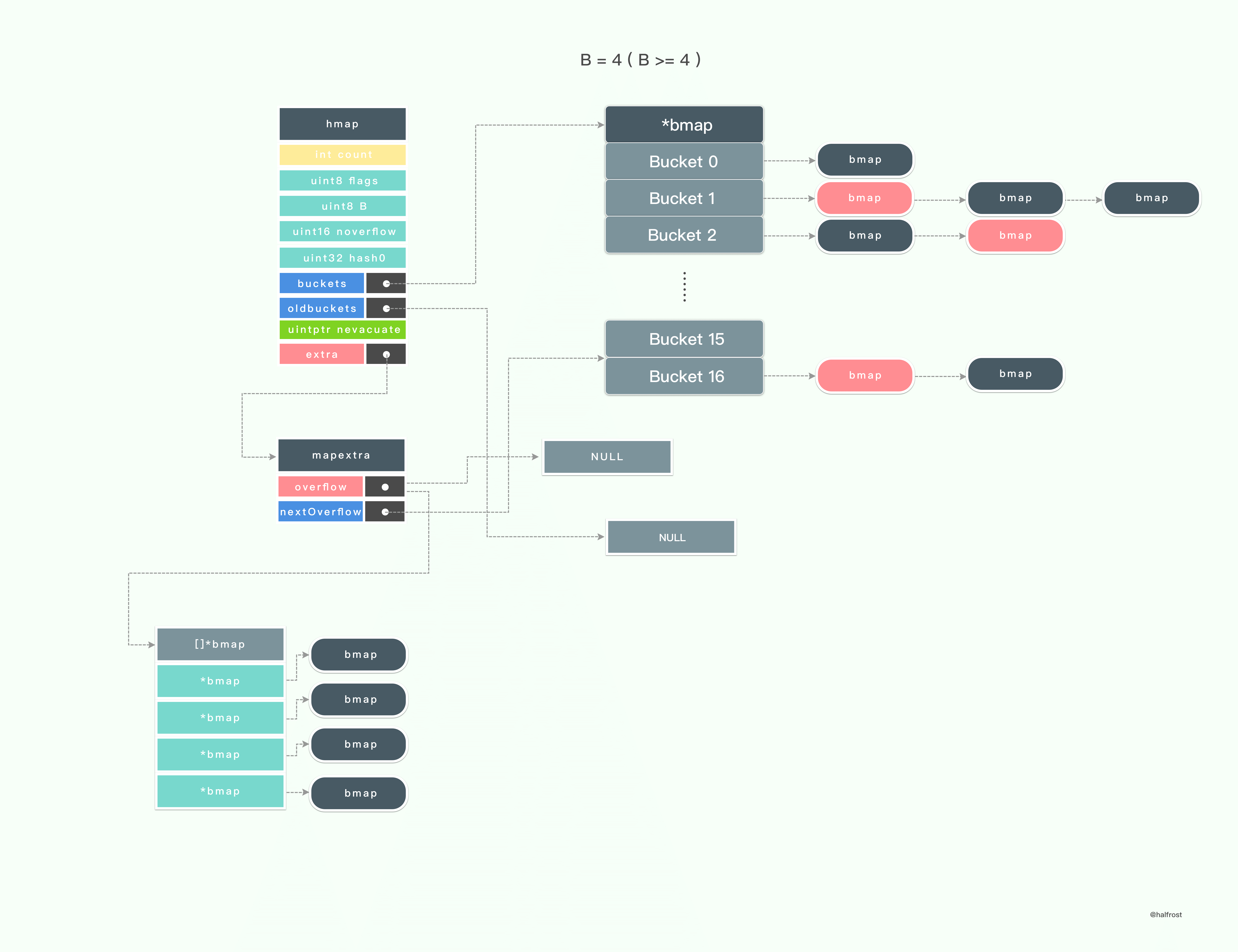
The final step is to release the old buckets and set the oldbuckets pointer to null. At this point, a migration process is fully complete.
5. Same-Size Grow
Strictly speaking, this approach cannot really be considered growth. But since the function name is Grow, we will call it that for now.
Starting with Go 1.8, sameSizeGrow was added. When the number of overflow buckets exceeds a certain threshold (2^B) but the load factor has not yet reached 6.5, there may be some empty buckets, meaning bucket utilization is low. In this case, sameSizeGrow is triggered: B remains unchanged, but the data migration process is still executed, compacting the data from oldbuckets to improve bucket utilization. Of course, during sameSizeGrow, loadFactorGrow will not be triggered.
IV. Some Optimizations in the Map Implementation
Having read this far, readers should have a clear idea of how to design and implement a Map, including the implementation of the various operations on a Map. Before exploring how to implement a thread-safe Map, let’s summarize some of the optimization highlights discussed earlier.
In Redis, incremental expansion is used to handle hash collisions. When the average lookup length exceeds 5, incremental expansion is triggered to ensure high performance of the hash table.
Redis also uses head insertion to ensure good performance when inserting key values.
In Java, once the number of buckets exceeds 64, and the number of colliding nodes is 8 or greater, conversion to a red-black tree is triggered. This ensures that even when the linked list is very long, the lookup length does not become too large, and the red-black tree guarantees O(log n) time complexity in the worst case.
Java has a very nice design after migration: it only needs to check whether the highest bit of the bucket count after migration is 0. If it is 0, the key’s relative position in the new bucket remains unchanged; if it is 1, adding the old bucket count oldCap gives the new position.
Go has quite a few optimizations:
- The hash algorithm uses the efficient memhash algorithm and CPU AES instruction set. The AES instruction set fully leverages CPU hardware characteristics, making hash computation extremely efficient.
- The key-value layout is designed so that keys are placed together and values are placed together, rather than storing key and value pairs side by side. This makes memory alignment easier and saves some of the waste caused by memory alignment when the data volume becomes large.
- When the memory size of a key or value exceeds 128 bytes, it is automatically converted to storing a pointer.
- The design of the tophash array accelerates key lookup. tophash is also reused to mark state during growth operations.
- Bit operations are used to transform modulo operations. For m % n, when n = 1 « B, it can be transformed into m & (1 « B - 1).
- Incremental growth.
- Same-size grow and compaction.
- Since Go 1.9, Map has natively supported thread safety. (This issue will be discussed in depth in the next chapter.)
Of course, there are still some areas in Go that could be further optimized:
- During migration, the current version does not reuse overflow buckets; instead, it directly allocates a new bucket. This could be optimized to preferentially reuse overflow buckets that are no longer pointed to by any pointer, and only allocate a new one when none are available. The author has already written this in the TODO.
- Dynamically merge multiple empty buckets.
- The current version has no shrink operation; a Map can only grow and cannot shrink. Redis has a related implementation for this.
(Given the length of a single article, the entire thread-safety section will be covered in the next article, which will be updated shortly.)
References:
Algorithms and Data Structures
Redis Design and Implementation
xxHash
String Hash Functions
General Purpose Hash Function Algorithms
Java 8 Series: Reacquainting Yourself with HashMap
GitHub Repo: Halfrost-Field
Follow: halfrost · GitHub
Source: https://halfrost.com/go_map/