How Is the CellID in Google S2 Generated?
In “Efficient Multidimensional Spatial Point Indexing Algorithms — Geohash and Google S2”, I analyzed the implementation ideas behind the Google S2 algorithm in detail. After the article was published, some readers became curious about its implementation. This article serves as a supplement to the previous one, looking at the concrete implementation of Google S2 from a code perspective. I recommend first reading the algorithmic ideas in the previous article; the code implementation in this article will then be easier to understand.
1. What Is a Cell?
Google S2 defines a framework for decomposing the unit sphere into a hierarchical structure of cells. Each Cell is a quadrilateral bounded by four geodesics. The top level of the hierarchy is obtained by projecting the six faces of a cube onto the unit sphere; lower levels are obtained by recursively subdividing each cell into four child cells. For example, the image below shows two Cells on one of the six faces, one of which has been subdivided several times:
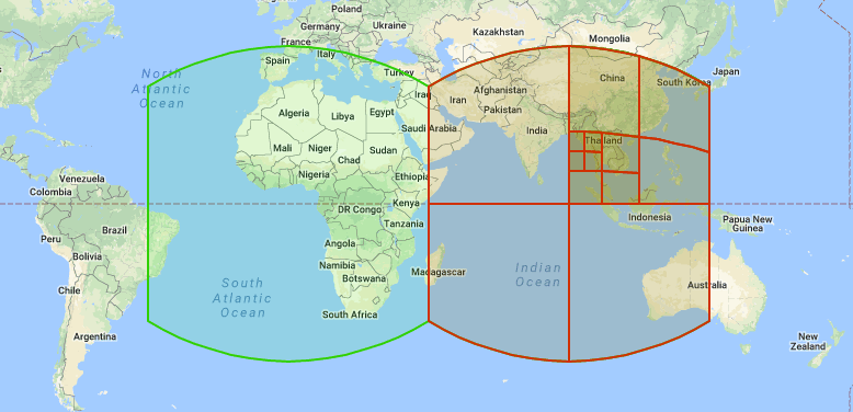
Note that the Cell edges appear curved because they are spherical geodesics—that is, straight lines on the sphere (similar to the routes airplanes fly).
Each cell in the hierarchy has a level, defined as the number of times the cell has been subdivided (starting from a face cell). Cell levels range from 0 to 30. The smallest cells at level 30 are called leaf cells; there are 6 * 4^30^ of them in total, each roughly 1 cm across on the Earth’s surface. (Details about cell sizes at each level can be found in S2 Cell ID Data Structure.)
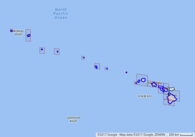
S2 Levels are very useful for spatial indexing and for approximating regions as collections of cells. Cells can be used to represent both points and regions: points are typically represented as leaf nodes, while regions are represented as collections of Cells at any Level. For example, the following is a collection of 22 cells approximating Hawaii:
2. S(lat,lng) -> f(x,y,z)
Latitude ranges from [-90°,90°].
Longitude ranges from [-180°,180°].
The first transformation converts spherical coordinates into three-dimensional Cartesian coordinates.
func makeCell() {
	latlng := s2.LatLngFromDegrees(30.64964508, 104.12343895)
	cellID := s2.CellIDFromLatLng(latlng)
}
The two short statements above construct a 64-bit CellID.
func LatLngFromDegrees(lat, lng float64) LatLng {
	return LatLng{s1.Angle(lat) * s1.Degree, s1.Angle(lng) * s1.Degree}
}
The step above converts latitude and longitude to radians. Since latitude and longitude are in degrees, converting degrees to radians only requires multiplying by π / 180°.
const (
	Radian Angle = 1
	Degree       = (math.Pi / 180) * Radian
}
LatLngFromDegrees converts latitude and longitude into a LatLng struct. The LatLng struct is defined as follows:
type LatLng struct {
	Lat, Lng s1.Angle
}
Once you have a LatLng struct, you can use the CellIDFromLatLng method to convert latitude/longitude radians into a 64-bit CellID.
func CellIDFromLatLng(ll LatLng) CellID {
	return cellIDFromPoint(PointFromLatLng(ll))
}
The method above is also completed in two steps: first convert the latitude and longitude into a point in the coordinate system, then convert that point in the coordinate system into a CellID.
For how to convert latitude and longitude into a point in the coordinate system, see the general analysis in this article. It explains, from a code implementation perspective, how to convert a point in a spherical coordinate system into the corresponding point on a Hilbert curve in a quadtree.
func PointFromLatLng(ll LatLng) Point {
	phi := ll.Lat.Radians()
	theta := ll.Lng.Radians()
	cosphi := math.Cos(phi)
	return Point{r3.Vector{math.Cos(theta) * cosphi, math.Sin(theta) * cosphi, math.Sin(phi)}}
}
The function above converts latitude and longitude into a vector point in a 3D coordinate system. The vector starts at the origin of the 3D coordinates and ends at the point converted onto the sphere. The conversion relationship is shown below:
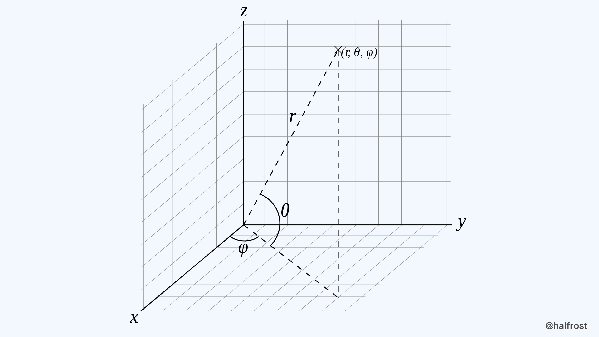
θ is the latitude in the longitude/latitude pair, which is phi in the code above; φ is the longitude, which is theta in the code above. Using trigonometric functions, we can obtain the 3D coordinates of this vector:
x = r * cos θ * cos φ
y = r * cos θ * sin φ
z = r * sin θ
The radius of the sphere in the figure is r = 1. Therefore, the resulting constructed vector is:
r3.Vector{math.Cos(theta) * cosphi, math.Sin(theta) * cosphi, math.Sin(phi)}
(x, y, z) is a direction vector; its components are not required to form a unit vector. The values of (x, y, z) lie within the 3D cube [-1,+1] x [-1,+1] x [-1,+1]. They can be normalized to obtain the corresponding point on the unit sphere.
At this point, the transformation from a point on the sphere S(lat,lng) -> f(x,y,z) has been completed.
III. f(x,y,z) -> g(face,u,v)
Next, perform the transformation f(x,y,z) -> g(face,u,v).
func xyzToFaceUV(r r3.Vector) (f int, u, v float64) {
	f = face(r)
	u, v = validFaceXYZToUV(f, r)
	return f, u, v
}
The idea here is to perform a projection.
First, choose the longest of the x, y, and z axes as the principal axis.
func (v Vector) LargestComponent() Axis {
	t := v.Abs()

	if t.X > t.Y {
		if t.X > t.Z {
			return XAxis
		}
		return ZAxis
	}
	if t.Y > t.Z {
		return YAxis
	}
	return ZAxis
}
By default, the x-axis is defined as 0, the y-axis as 1, and the z-axis as 2.
const (
	XAxis Axis = iota
	YAxis
	ZAxis
)
Finally, the value of face is the longest of the three axes. Note that all three are constrained to the range [0,5], so if it is a negative axis, you need to add 3 to correct it. The implementation is as follows.
func face(r r3.Vector) int {
	f := r.LargestComponent()
	switch {
	case f == r3.XAxis && r.X < 0:
		f += 3
	case f == r3.YAxis && r.Y < 0:
		f += 3
	case f == r3.ZAxis && r.Z < 0:
		f += 3
	}
	return int(f)
}
Thus, the values for the six faces are determined: when the principal axis is the positive x-axis, face = 0; when the principal axis is the positive y-axis, face = 1; when the principal axis is the positive z-axis, face = 2; when the principal axis is the negative x-axis, face = 3; when the principal axis is the negative y-axis, face = 4; and when the principal axis is the negative z-axis, face = 5.
After selecting the principal axis, you need to project the coordinate points on the other two axes onto this face. In practice, this is done through projection or a coordinate-system transformation.
func validFaceXYZToUV(face int, r r3.Vector) (float64, float64) {
	switch face {
	case 0:
		return r.Y / r.X, r.Z / r.X
	case 1:
		return -r.X / r.Y, r.Z / r.Y
	case 2:
		return -r.X / r.Z, -r.Y / r.Z
	case 3:
		return r.Z / r.X, r.Y / r.X
	case 4:
		return r.Z / r.Y, -r.X / r.Y
	}
	return -r.Y / r.Z, -r.X / r.Z
}
The above describes the coordinate-system transformations on the 6 faces. If you map them intuitively to the 6 faces of a circumscribed cube, then face = 0 corresponds to the front face, face = 1 to the right face, face = 2 to the top face, face = 3 to the back face, face = 4 to the left face, and face = 5 to the bottom face.
Note that the 3D coordinate axes here follow a right-handed coordinate system. That is, if the four fingers of your right hand curl in the direction from the x-axis to the y-axis, your thumb points in the positive direction of the other face.
For example, on the front face of the cube, when the right hand rotates from the positive direction of the y-axis to the positive direction of the z-axis, the thumb points in the positive direction of the x-axis, so it corresponds to the front face. As another example, on the bottom face of the cube, when the right hand rotates from the negative direction of the y-axis to the negative direction of the x-axis, the thumb points in the negative direction of the z-axis, so it corresponds to the bottom face.
(face,u,v) represents a cubic-space coordinate system, where the value range of all three axes is [-1,1]. To make every cell the same size, a transformation is required; the specific transformation rules are covered in the next conversion step.
IV. g(face,u,v) -> h(face,s,t)
The conversion from u, v to s, t uses a quadratic transform. In the C++ version, there are three kinds of transforms. As for why this quadratic transform was ultimately chosen, see here.
// Linear transform
u = 0.5 * ( u + 1)

// tan() transform
u = 2 / pi * (atan(u) + pi / 4) = 2 * atan(u) / pi + 0.5

// Quadratic transform
u >= 0,u = 0.5 * sqrt(1 + 3*u)
u < 0, u = 1 - 0.5 * sqrt(1 - 3*u)
In Go, the transformation only includes the quadratic transform; the other two transforms simply have no corresponding code in the Go implementation.
func uvToST(u float64) float64 {
	if u >= 0 {
		return 0.5 * math.Sqrt(1+3*u)
	}
	return 1 - 0.5*math.Sqrt(1-3*u)
}
(face,s,t) represents a cell-space coordinate system, where the ranges of s and t are both [0,1]. They represent a point on a face. For example, the point (s,t) = (0.5,0.5) represents the center point on this face. This point is also the vertex formed when the current face is subdivided into 4 smaller cells.
V. h(face,s,t) -> H(face,i,j)
This section covers coordinate-system conversion. For the underlying idea, see here.
Convert a point in s and t coordinates into a point in the i and j coordinate system.
func stToIJ(s float64) int {
	return clamp(int(math.Floor(maxSize*s)), 0, maxSize-1)
}
The value ranges of s and t are [0,1]; now the range needs to be expanded to [0,2^30^-1]. This is only one face.
6. H(face,i,j) -> CellID
Before performing the final conversion, let’s first review the conversion process so far.
func CellIDFromLatLng(ll LatLng) CellID {
    return cellIDFromPoint(PointFromLatLng(ll))
}

func cellIDFromPoint(p Point) CellID {
	f, u, v := xyzToFaceUV(r3.Vector{p.X, p.Y, p.Z})
	i := stToIJ(uvToST(u))
	j := stToIJ(uvToST(v))
	return cellIDFromFaceIJ(f, i, j)
}
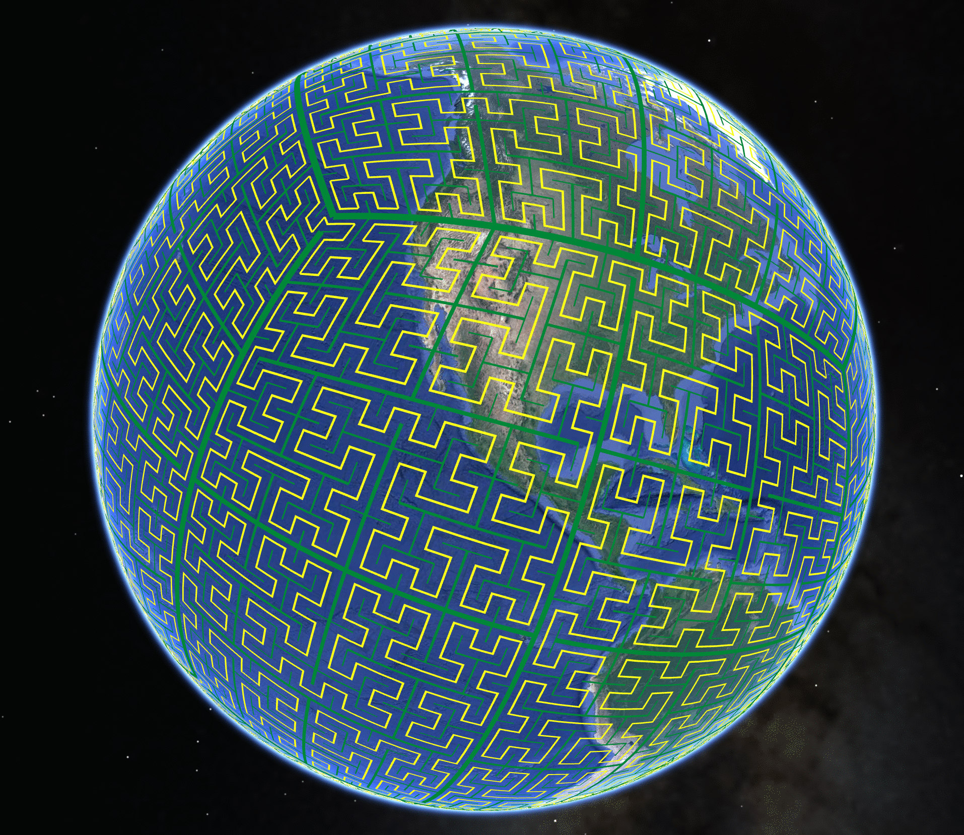
S(lat,lng) -> f(x,y,z) -> g(face,u,v) -> h(face,s,t) -> H(face,i,j) -> CellID involves a total of 5 transformation steps.
After these 5 transformations, this is equivalent to mapping every latitude/longitude point on Earth to a point on the Hilbert curve.
Before explaining the final transformation to CellID, let’s first clarify the issue of orientation.
There are 2 arrays that store constants:
	ijToPos = [4][4]int{
		{0, 1, 3, 2}, // canonical order
		{0, 3, 1, 2}, // axes swapped
		{2, 3, 1, 0}, // bits inverted
		{2, 1, 3, 0}, // swapped & inverted
	}
	posToIJ = [4][4]int{
		{0, 1, 3, 2}, // canonical order:    (0,0), (0,1), (1,1), (1,0)
		{0, 2, 3, 1}, // axes swapped:       (0,0), (1,0), (1,1), (0,1)
		{3, 2, 0, 1}, // bits inverted:      (1,1), (1,0), (0,0), (0,1)
		{3, 1, 0, 2}, // swapped & inverted: (1,1), (0,1), (0,0), (1,0)
	}
The values in these two two-dimensional arrays are illustrated in the following two figures:
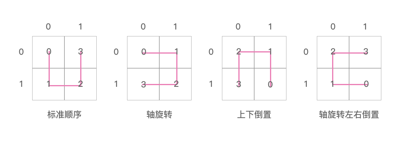
The figure above is posToIJ. Note that i and j here refer to coordinate values, as shown above. This is a first-order Hilbert curve, so i and j are equal to the values on the coordinate axes. posToIJ[0] = {0, 1, 3, 2} represents what is shown in diagram 0 above. Similarly, posToIJ[1] represents diagram 1, posToIJ[2] represents diagram 2, and posToIJ[3] represents diagram 3.
From the four diagrams above, we can see that:
The four diagrams of posToIJ are actually obtained by rotating a “U” shape counterclockwise by 90° each time. Here we can only see the relationships among the four diagrams—that is, the sibling relationships—but we cannot see the relationships between parent and child diagrams.
The values stored in posToIJ[0] = {0, 1, 3, 2} are the combined ij values. posToIJ[0][0] = 0 refers to the cell where i = 0 and j = 0; combined as ij, this is 00, i.e. 0. posToIJ[0][1] = 1 refers to the cell where i = 0 and j = 1; combined as ij, this is 01, i.e. 1. posToIJ[0][2] = 1 refers to the cell where i = 1 and j = 1; combined as ij, this is 11, i.e. 3. posToIJ[0][3] = 2 refers to the cell where i = 1 and j = 0; combined as ij, this is 10, i.e. 2. The order in the array is the order in which the “U” shape is drawn. Therefore, posToIJ[0] = {0, 1, 3, 2} represents what is shown in diagram 0. The same applies to the other diagrams.
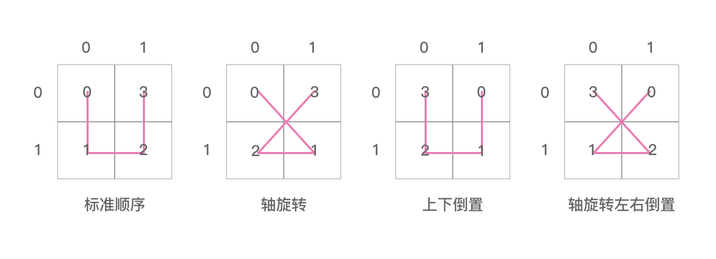
The four diagrams above are for the ijToPos array. This array is not used anywhere in the entire library, so there is no need to worry about its corresponding relationship here.
The lookupPos array and lookupIJ array are initialized by the following code.
func init() {
	initLookupCell(0, 0, 0, 0, 0, 0)
	initLookupCell(0, 0, 0, swapMask, 0, swapMask)
	initLookupCell(0, 0, 0, invertMask, 0, invertMask)
	initLookupCell(0, 0, 0, swapMask|invertMask, 0, swapMask|invertMask)
}
If we substitute all the variable values, the code becomes as follows:
func init() {
	initLookupCell(0, 0, 0, 0, 0, 0)
	initLookupCell(0, 0, 0, 1, 0, 1)
	initLookupCell(0, 0, 0, 2, 0, 2)
	initLookupCell(0, 0, 0, 3, 0, 3)
}
initLookupCell takes six parameters, four of which are 0. We need to focus on the fourth and sixth parameters. The fourth parameter is origOrientation, and the sixth parameter is orientation.
Inside the initLookupCell method, there are the following four lines:
initLookupCell(level, i+(r[0]>>1), j+(r[0]&1), origOrientation, pos, orientation^posToOrientation[0])
initLookupCell(level, i+(r[1]>>1), j+(r[1]&1), origOrientation, pos+1, orientation^posToOrientation[1])
initLookupCell(level, i+(r[2]>>1), j+(r[2]&1), origOrientation, pos+2, orientation^posToOrientation[2])
initLookupCell(level, i+(r[3]>>1), j+(r[3]&1), origOrientation, pos+3, orientation^posToOrientation[3])
As an aside, let’s explain what r[0]>>1 and r[0]&1 actually do.
r := posToIJ[orientation]
The r array comes from the posToIJ array. As mentioned earlier, the posToIJ array actually contains four “U” shapes in different directions. In effect, it represents the relative directions among the current four small sibling squares. What r[0], r[1], r[2], and r[3] retrieve are the four values 00, 01, 10, and 11. Therefore, the operation r[0]>>1 extracts the first bit of the two-bit binary value, i.e. the i bit. The operation r[0]&1 extracts the second bit of the two-bit binary value, i.e. the j bit. The same applies to r[1], r[2], and r[3].
Returning to the topic of direction, the first thing to clarify is what the following four lines do.
orientation^posToOrientation[0]
orientation^posToOrientation[1]
orientation^posToOrientation[2]
orientation^posToOrientation[3]
Before explaining further, let’s first take a look at the posToOrientation array:
posToOrientation = [4]int{swapMask, 0, 0, invertMask | swapMask}
Substitute the values into the array above:
posToOrientation = [4]int{1, 0, 0, 3}
The original values stored in the posToOrientation array are [01, 00, 00, 11]. These four values are not initialized arbitrarily.
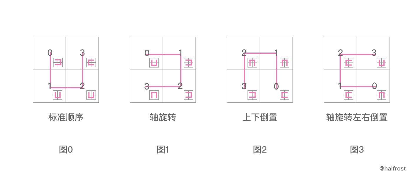
In fact, they correspond to the directions in which the four small squares in Figure 0 will be subdivided next. For position 0 in Figure 0, the direction of the next figure should be Figure 1, i.e. 01; for position 1 in Figure 0, the direction of the next figure should be Figure 0, i.e. 00; for position 2 in Figure 0, the direction of the next figure should be Figure 0, i.e. 00; and for position 3 in Figure 0, the direction of the next figure should be Figure 3, i.e. 11. This is the trick behind the initialization of the posToOrientation array.
From the four diagrams for posToIJ, we can only see the relationships among siblings, whereas the four diagrams for posToOrientation tell us about the parent-child relationships.
Returning to the code mentioned above:
orientation^posToOrientation[0]
orientation^posToOrientation[1]
orientation^posToOrientation[2]
orientation^posToOrientation[3]
XOR the orientation with the posToOrientation array each time. This ensures that, each time, the current direction of pos can be derived from the previous original direction. In other words, it computes the relationship between parent and child.
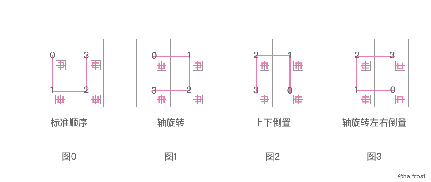
Let’s return to this diagram. The relationship between siblings is a 90° counterclockwise rotation. So, when these four siblings each become parents, what is the relationship between each of them and their four children? The conclusion is: the parent-child relationships are 01, 00, 00, 11. We can also see this from the diagram. In Figure 1, although the “U” shape has been rotated 90° counterclockwise, its children have also rotated 90° with it (relative to Figure 0). The same is true for Figures 2 and 3.
In code, this relationship is represented by the following four lines:
orientation^posToOrientation[0]
orientation^posToOrientation[1]
orientation^posToOrientation[2]
orientation^posToOrientation[3]
For example, suppose orientation = 0, i.e., Figure 0; then:
00 ^ 01 = 01
00 ^ 00 = 00
00 ^ 00 = 00
00 ^ 11 = 11
The directions of the four children in Figure 0 have been calculated: 01, 00, 00, 11, 1003. This is consistent with what Figure 0 shows in the image above.
The same reasoning applies to orientation = 1, orientation = 2, and orientation = 3:
01 ^ 01 = 00
01 ^ 00 = 01
01 ^ 00 = 01
01 ^ 11 = 10


10 ^ 01 = 11
10 ^ 00 = 10
10 ^ 00 = 10
10 ^ 11 = 01

11 ^ 01 = 10
11 ^ 00 = 11
11 ^ 00 = 11
11 ^ 11 = 00
In Figure 1, the children’s orientations are 0, 1, 1, 2. In Figure 2, the children’s orientations are 3, 2, 2, 1. In Figure 3, the children’s orientations are 2, 3, 3, 0. This is completely consistent with what is drawn in the figures.
So the conversion above is critical. This is where the parent-child orientation conversion for the Hilbert curve is performed.
Finally, some readers may wonder: what is the relationship between origOrientation and orientation?
lookupPos[(ij<<2)+origOrientation] = (pos << 2) + orientation
lookupIJ[(pos<<2)+origOrientation] = (ij << 2) + orientation
What is stored in the array indices is origOrientation, while the values stored at those indices are orientation.
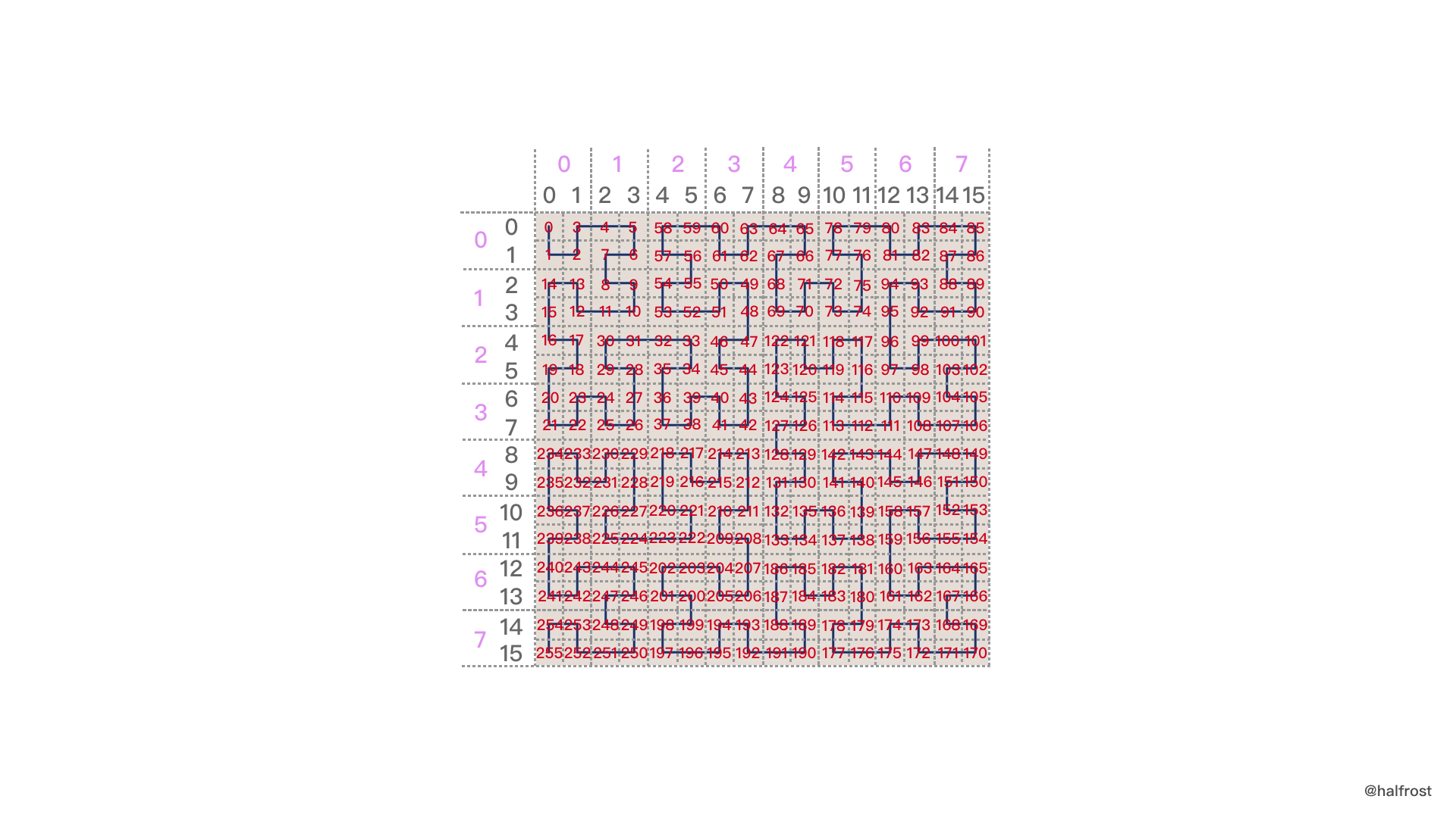
After explaining the issue of Hilbert curve orientation, we can now take a closer look at the coordinate conversion problem for 55. This was discussed in the previous article, “Efficient Multidimensional Spatial Point Indexing Algorithms — Geohash and Google S2”, but some readers still had questions, so here is a final explanation.
In Google S2, when initLookupCell is initialized, two arrays are initialized: the lookupPos array and the lookupIJ array. Four key variables are also used in the process: i, j, pos, and orientation. orientation was already covered earlier, so I will not repeat it here. What needs to be explained in detail is the relationship between i, j, and pos.
pos refers to the position on the Hilbert curve. This position is counted from the starting point of the Hilbert curve: count from the start to determine which block the current one is. Note that this block is a large block composed of 4 smaller blocks, because orientation selects one of the 4 blocks.
In the example of 55, pos is actually equal to 13. It means that the current large block composed of 4 small blocks is the 13th large block from the starting point. Since each large block consists of 4 small blocks, the first number in the current large block is 13 * 4 = 52. In code, this is implemented by shifting left by 2 bits, which is equivalent to multiplying by 4. Then add the offset orientation = 11 for 55, i.e. add 3, so 52 + 3 = 55.
Now let’s talk about i and j. In the example of 55, i = 14, 1110, and j = 13, 1101. If you look at the coordinate system intuitively, 55 is actually at coordinate (5, 2). So why are i = 14 and j = 13 here? What is easy to confuse is the relationship between i, j, and pos.
Note:
i and j do not directly correspond to coordinates in the Hilbert curve coordinate system. This is because the initialization needs to generate a fifth-order Hilbert curve. In the first-order Hilbert curve represented by the posToIJ array, i and j directly correspond to coordinates in the Hilbert curve coordinate system.
At this point, readers may wonder: then which parameter corresponds to the coordinates in the Hilbert curve coordinate system?
The pos parameter corresponds to the coordinates in the Hilbert curve coordinate system. Once the starting point and order of a Hilbert curve are determined, and once the pos position of a large block composed of four small blocks is determined, its coordinates are in fact already determined. Coordinates on the Hilbert curve do not depend on i or j; they are entirely determined by the properties of the curve and the pos position.
We do not care about the coordinates of small blocks on the Hilbert curve. What we care about is the conversion relationship between pos and i, j!
Another question arises: what coordinate system do i and j correspond to?
i and j correspond to coordinates in a coordinate system after a coordinate transformation.
We know that when performing the ( u,v ) -> ( i,j ) transformation, the value range of u and v is [0,1], and after the transformation they are mapped into [ 0, 2^30^-1 ]. i and j are the coordinate values in the transformed coordinate system, and their value range becomes [ 0, 2^30^-1 ].
So what is the purpose of initializing and computing the lookupPos and lookupIJ arrays? These two arrays are what connect i, j, and pos. Once you know pos, you can immediately find the corresponding i and j. Once you know i and j, you can immediately find the corresponding pos.
The bridge for converting between i, j, and pos is the way the Hilbert curve is generated. This method can be compared to the way a Z-index curve is generated.
The way a Z-index curve is generated is to bisect the longitude and latitude coordinate intervals separately: the left interval is recorded as 0, and the right interval as 1. In the two resulting binary strings, even-numbered bits are assigned to longitude and odd-numbered bits to latitude. They are then combined into a new binary string, and after base-32 encoding, the final geohash is produced.
So how is a Hilbert curve generated? First, longitude and latitude coordinates are converted into coordinates in a 3D Cartesian coordinate system, then projected onto the 6 faces of the circumscribed cube. Thus the 3D Cartesian coordinates (x,y,z) are converted into (face,u,v). (face,u,v) undergoes a quadratic transform to become (face,s,t), and (face,s,t) undergoes a coordinate-system transformation to become (face,i,j). Then i and j are each extracted 4 bits at a time: the 4 binary bits of i go first, and the 4 binary bits of j go after them. Finally, add the 2 orientation bits orientation. This forms a 10-bit binary value like iiii jjjj oo. Through the bridge of the lookupPos array, the corresponding pos value is found. The pos value is the corresponding position on the Hilbert curve. The same process continues: take another 4 bits from i and another 4 bits from j and convert them in this way until all binary bits of i and j have been consumed. Finally, concatenate the generated pos values into the final CellID, placing the earlier-generated values in the high bits and the later-generated values in the low bits.
Some readers may wonder why it is designed as
iiii jjjj oo, and why 4 bits are taken at a time. Google developers wrote the following in the comments: “We once considered combining 16 bits at a time: 14 bits of position + 2 bits of orientation. But when the code actually ran, we found that smaller arrays had better performance, and 2KB was more suitable for storage in the primary cache.”
In Google S2, i and j are converted 4 bits at a time, so the valid values of i and j are 0–15. Therefore, iiii jjjj oo is a decimal number whose representable range is 2^10^ = 1024. Then the initial values of pos also need to be computed up to 1024. Since pos is a large block composed of 4 small blocks, it is itself a first-order Hilbert curve. Therefore, initialization needs to generate a fifth-order Hilbert curve.
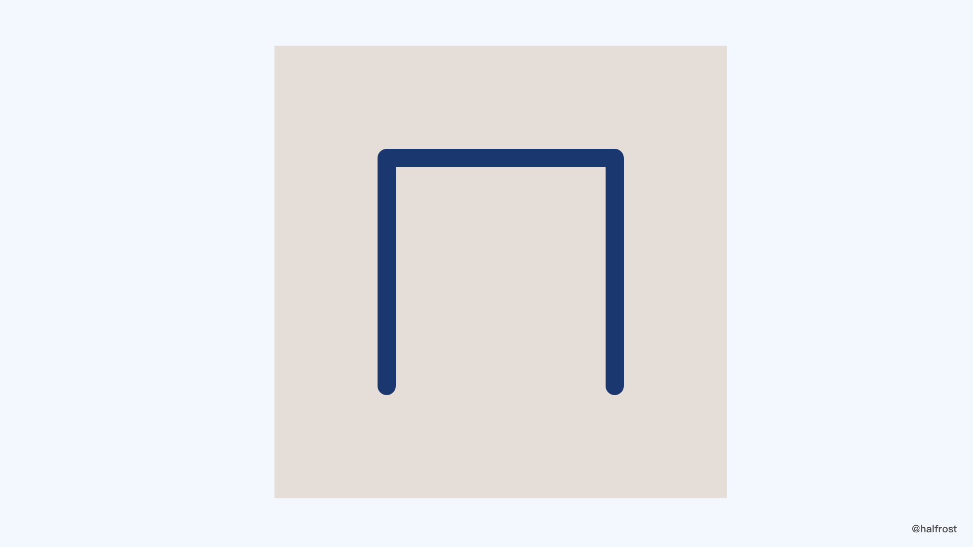
The figure above is a first-order Hilbert curve. It consists of 4 small squares.
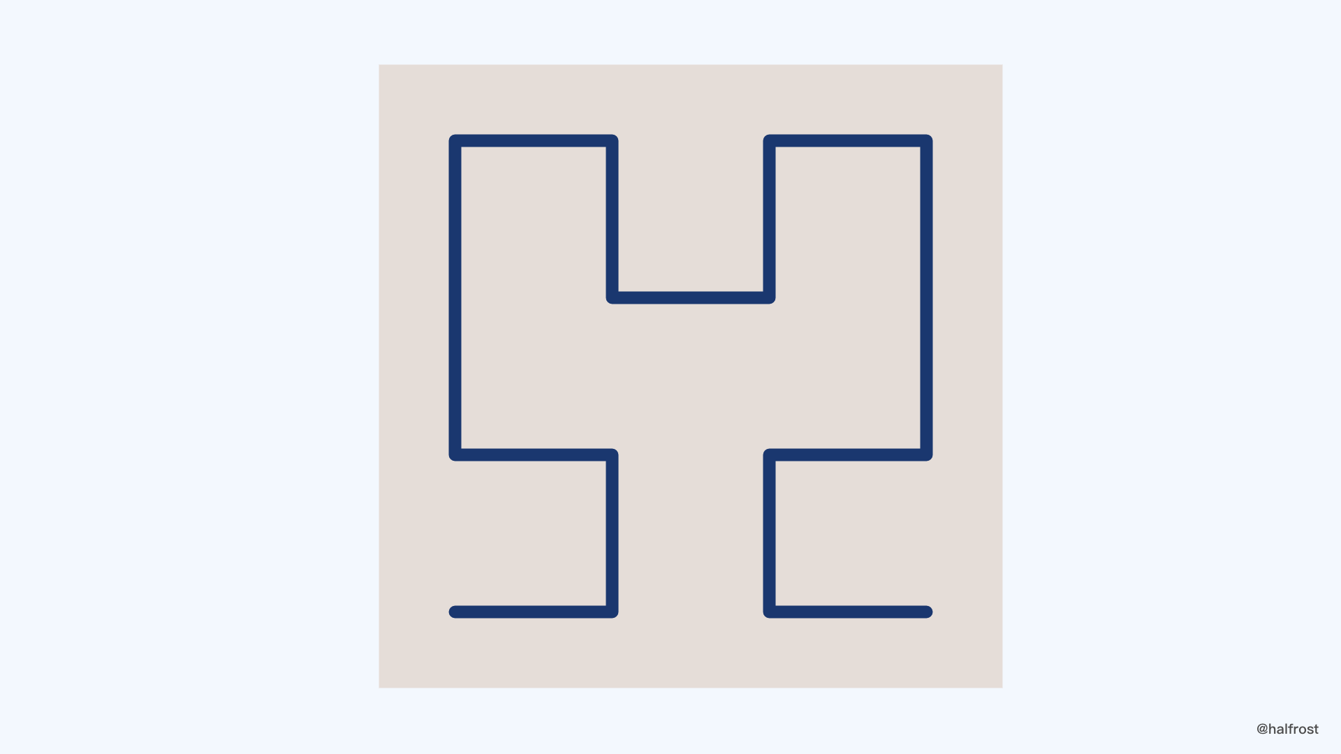
The figure above is a second-order Hilbert curve, consisting of 4 pos squares.
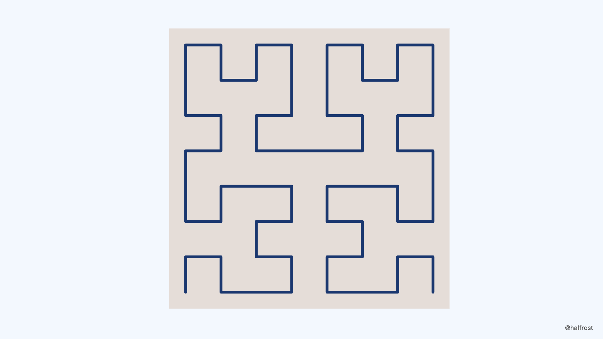
The figure above is a third-order Hilbert curve.
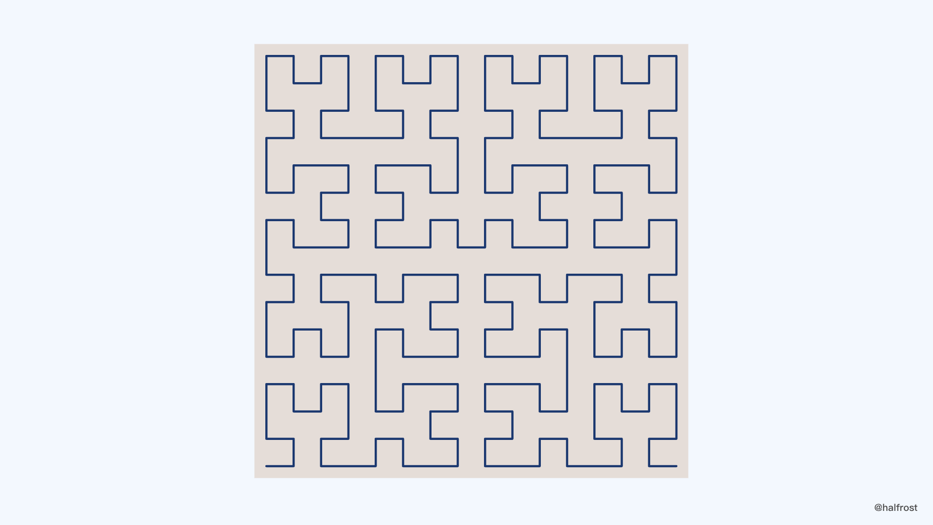
The figure above is a fourth-order Hilbert curve.
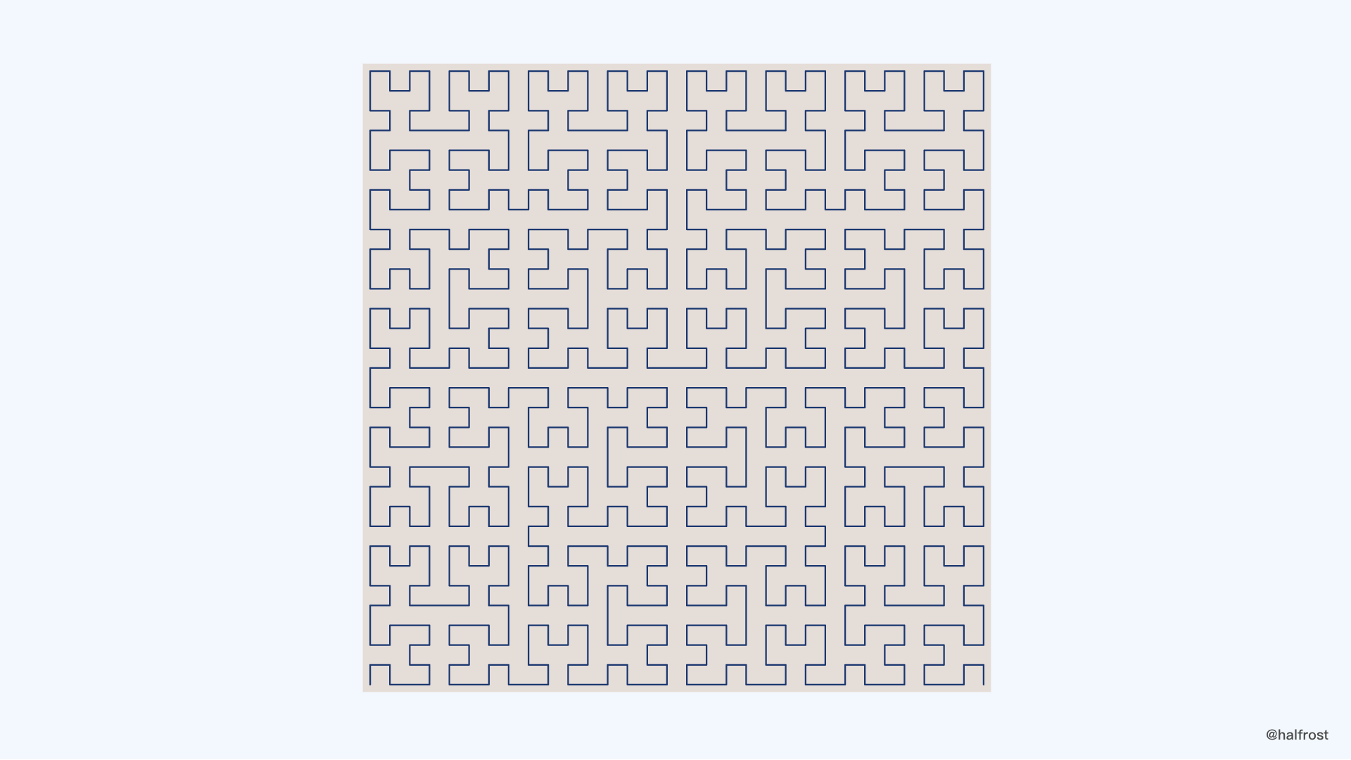
The figure above is a fifth-order Hilbert curve. There are 1024 pos squares in total.
At this point, we have clarified the orientation of the Hilbert curve and the order of the Hilbert curve generated in Google S2: a fifth-order Hilbert curve.
From this, we can also see that the Hilbert curve is composed of “U” shapes, specifically of four “U” shapes in different orientations. The initial orientation is a “U” with its opening facing upward.
For an animation of Hilbert curve generation, see the previous article’s section “Efficient Multidimensional Spatial Point Indexing Algorithms — Geohash and Google S2” — Construction Method of the Hilbert Curve.
Now calculating 55 becomes relatively simple. Start from the fifth-order Hilbert curve and work through it as shown below.
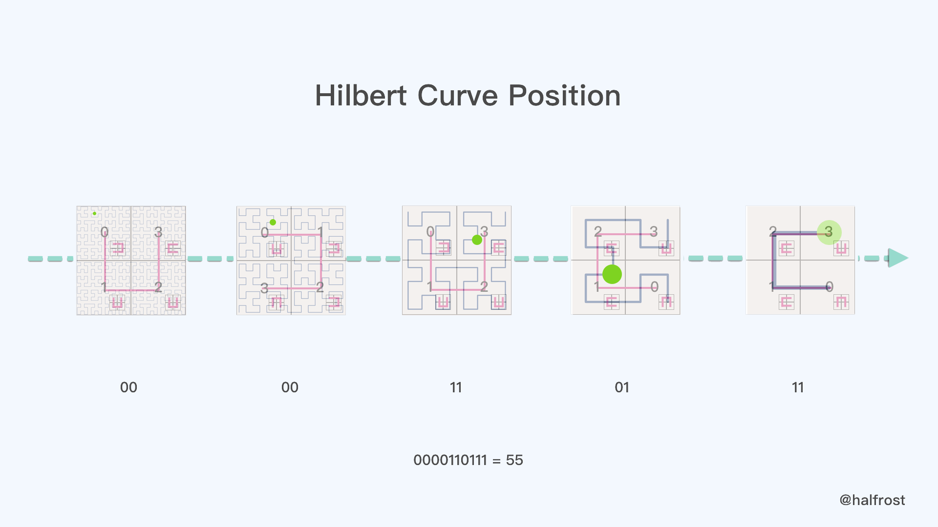
First, 55 is at the green point in each small diagram in the figure above. We continuously determine the orientation. In the first small diagram, the green point is at position 00. In the second small diagram, the green point is at position 00. In the third small diagram, the green point is at position 11. In the fourth small diagram, the green point is at position 01. In the fifth small diagram, the green point is at position 11. In fact, after converting to the fourth step, the resulting value is the value of pos, namely 00001101 = 13. The last 2 bits are the position of the specific point inside the pos square, which is 11, so 13 * 4 + 3 = 55.
Of course, if you directly derive it all the way according to the orientations, you can also obtain 0000110111 = 55, which is likewise 55.
VII. Example
Finally, here is a complete concrete example:
Since Ghost does not support tables, please see the table on my GitHub
The first 4 conversion steps have been completed above.
The final step is converting to CellID. The concrete implementation code is as follows. Since CellID is 64 bits, after excluding the 3 bits occupied by face and the position occupied by the final marker bit 1, 60 bits remain.
func cellIDFromFaceIJ(f, i, j int) CellID {
  // 1.
	n := uint64(f) << (posBits - 1)
  // 2.
	bits := f & swapMask
  // 3.
	for k := 7; k >= 0; k-- {
		mask := (1 << lookupBits) - 1
		bits += int((i>>uint(k*lookupBits))&mask) << (lookupBits + 2)
		bits += int((j>>uint(k*lookupBits))&mask) << 2
		bits = lookupPos[bits]
    // 4.
		n |= uint64(bits>>2) << (uint(k) * 2 * lookupBits)
    // 5.
		bits &= (swapMask | invertMask)
	}
  // 6.
	return CellID(n*2 + 1)
}
The specific steps are as follows:
- Shift face left by 60 bits.
- Compute the initial origOrientation. The initial origOrientation is derived from face, and the result after face & 01 is used to give each face a right-handed coordinate system.
- Loop from the beginning, taking the 4-bit binary values of i and j in order, compute ij«2 + origOrientation, then look up the corresponding pos«2 + orientation in the lookupPos array.
- Concatenate the CellID: shift pos«2 + orientation right by 2 bits, leaving only pos, then concatenate pos to the CellID from the previous loop.
- Compute the origOrientation for the next iteration. &= (swapMask | invertMask), that is, & 11, which extracts the last 2 binary bits.
- Finally, append the last marker bit 1.
Here, let’s discuss step 2: the conversion of origOrientation.
We know that face has 6 faces, numbered 000, 001, 010, 011, 100, and 101. To make all 6 faces satisfy the properties of a right-handed coordinate system, a conversion must be performed. The conversion rule is actually just a bitwise operation:
000 & 001 = 00
001 & 001 = 01
010 & 001 = 00
011 & 001 = 01
100 & 001 = 00
101 & 001 = 01
After the conversion, the value of face & 01 is the initial origOrientation.
The following table shows each step (the table is fairly long; swipe right to view):
Since Ghost does not support tables, please see the table on my GitHub
Pick any one case from the loop; represented as a diagram, it looks like this:
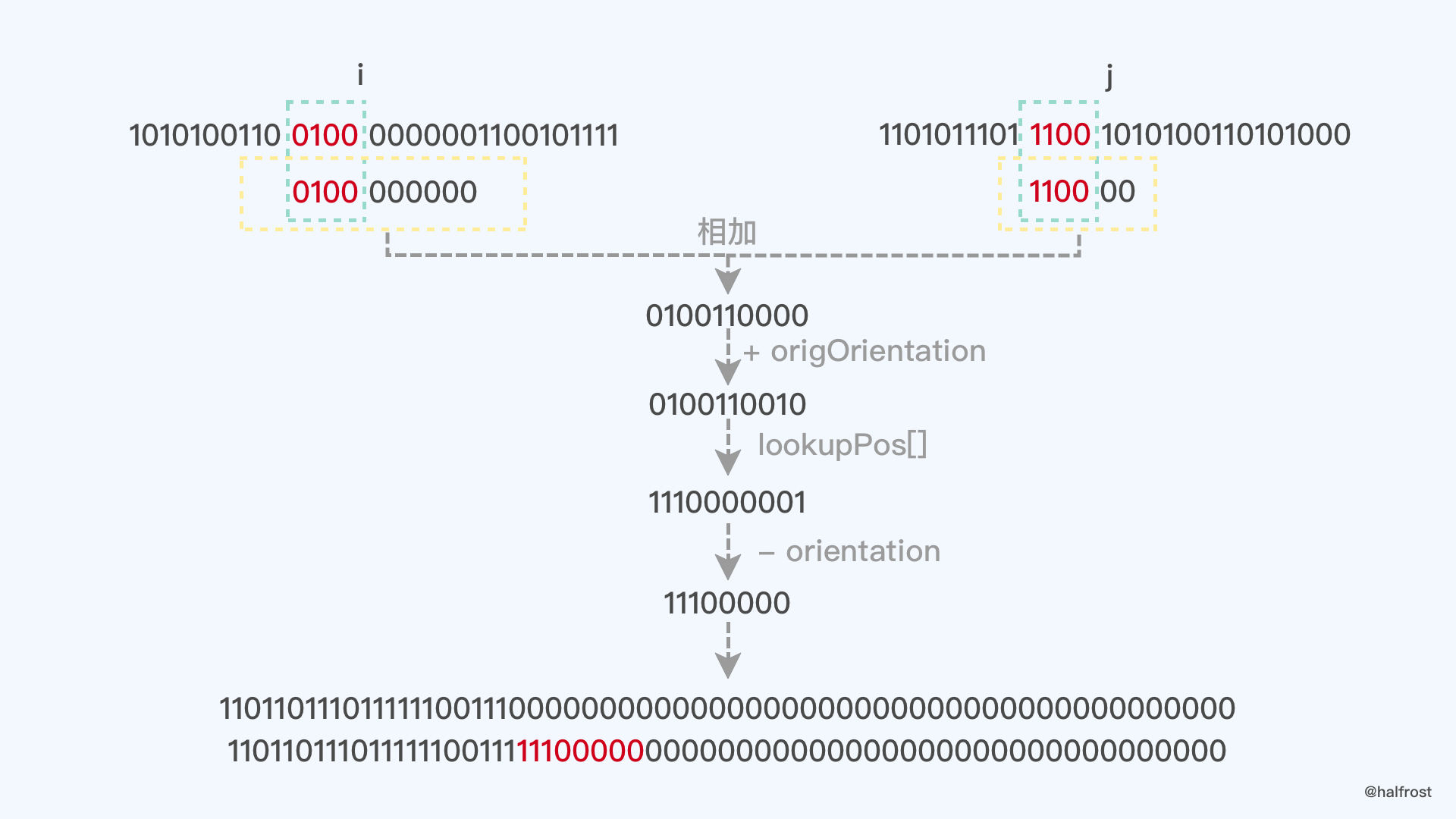
Note: Since CellID is 64 bits, the first three bits are face, and the last bit is the flag bit, so there are 60 bits in the middle. i and j are 30 bits when converted to binary: seven 4-bit binary groups and one 2-bit binary group. 4*7 + 2 = 30. iijjoo—that is, the first 2 binary bits of i and the first 2 binary bits of j, plus origOrientation—forms a 6-bit binary value, which can represent at most 2^6^ = 32 values. The converted pos + orientation is therefore at most 32 values as well. In other words, the converted result is at most 6 binary bits; after removing the last 2 bits for orientation, pos is at most 4 bits in this case. iiiijjjjpppp—that is, the 4 binary bits of i and the 4 binary bits of j, plus origOrientation—forms a 10-bit binary value, which can represent at most 2^10^ = 1024 values. The converted pos + orientation is therefore at most 10 bits. In other words, the converted result is at most 10 binary bits; after removing the last 2 bits for orientation, pos is at most 8 bits in this case.
Since the final CellID only concatenates pos, we get 4 + 7 * 8 = 60 bits. After concatenation is complete, the middle 60 bits are all composed of pos. Finally, append the first 3 bits and the trailing 1-bit flag, and the 64-bit CellID is generated.
At this point, the entire CellID generation process is complete.
Spatial search series:
Understanding n-dimensional space and n-dimensional spacetime
Efficient multidimensional point indexing algorithms — Geohash and Google S2
How Is CellID Generated in Google S2?
Computing the LCA (Lowest Common Ancestor) in Google S2’s Quadtree
The Magical De Bruijn Sequence
GitHub Repo:Halfrost-Field
Follow: halfrost · GitHub