How to Find Hilbert Curve Neighbors on a Quadtree?
Regarding the definition of neighbors: adjacent cells are neighbors, and neighbors can be divided into two types: edge-adjacent and vertex-adjacent. Edge-adjacent neighbors exist in four directions: up, down, left, and right. Vertex-adjacent neighbors also exist in four directions, corresponding to the four adjacent vertices.
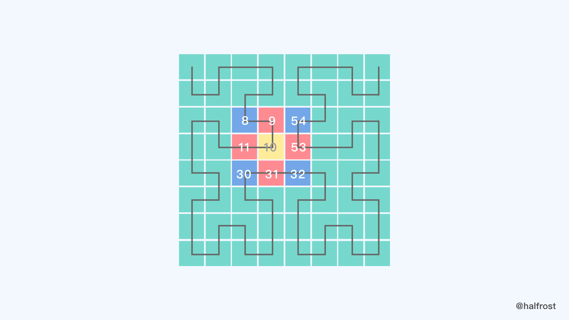
As shown above, the green area is the region represented by a quadtree, and there is a point on the quadtree—the point marked by the yellow area in the figure. We now want to find the Hilbert-curve neighbors of the yellow point on the quadtree. The black line in the figure is a Hilbert curve passing through the quadtree. The starting point 0 of the Hilbert curve is in the upper-left cell, and the ending point 63 is in the upper-right cell.
The four red cells are the edge-adjacent neighbors of the yellow cell, and the four blue cells are the vertex-adjacent neighbors of the yellow cell. Therefore, the yellow cell has eight neighboring cells, corresponding to the points 8, 9, 54, 11, 53, 30, 31, and 32. As you can see, these neighbors are not necessarily adjacent in terms of their point values.
So how do we find the Hilbert-curve neighbors of an arbitrary point on a quadtree?
I. Edge Neighbors
The most direct idea for edge neighbors is to first obtain the coordinates (i, j) of the center point, and then, based on the coordinate system, obtain the coordinates of the edge-adjacent Cells: (i + 1, j), (i - 1, j), (i, j - 1), and (i, j + 1).
The actual approach is the same. However, this involves a conversion step. We need to convert the point on the Hilbert curve into coordinates before we can compute edge neighbors using the approach above.
For the generation and data structure of CellID, see the author’s article “How Is CellID Generated in Google S2?”
Following the idea above, the implemented code is as follows:
func (ci CellID) EdgeNeighbors() [4]CellID {
	level := ci.Level()
	size := sizeIJ(level)
	f, i, j, _ := ci.faceIJOrientation()
	return [4]CellID{
		cellIDFromFaceIJWrap(f, i, j-size).Parent(level),
		cellIDFromFaceIJWrap(f, i+size, j).Parent(level),
		cellIDFromFaceIJWrap(f, i, j+size).Parent(level),
		cellIDFromFaceIJWrap(f, i-size, j).Parent(level),
	}
}
The edges are numbered 0, 1, 2, and 3 in counterclockwise order: bottom, right, top, and left.
Next, let’s take a closer look at the implementation.
func sizeIJ(level int) int {
	return 1 << uint(maxLevel-level)
}
sizeIJ stores the side length of a cell at the current Level. This size is relative to Level 30. For example, if level = 29, then its sizeIJ is 2, meaning that the side length of a Level 29 cell consists of 2 Level 30 cells; in other words, it consists of 2^2^=4 small cells. If level = 28, then the side length is 4, consisting of 16 small cells. The same logic applies to the other levels.
func (ci CellID) faceIJOrientation() (f, i, j, orientation int) {

	f = ci.Face()
	orientation = f & swapMask
	nbits := maxLevel - 7*lookupBits // first iteration

	for k := 7; k >= 0; k-- {
		orientation += (int(uint64(ci)>>uint64(k*2*lookupBits+1)) & ((1 << uint((2 * nbits))) - 1)) << 2
		orientation = lookupIJ[orientation]
		i += (orientation >> (lookupBits + 2)) << uint(k*lookupBits)
		j += ((orientation >> 2) & ((1 << lookupBits) - 1)) << uint(k*lookupBits)
		orientation &= (swapMask | invertMask)
		nbits = lookupBits // following iterations
	}
	// Detailed explanation of the following check
	if ci.lsb()&0x1111111111111110 != 0 {
		orientation ^= swapMask
	}
	return
}
This method decomposes a CellID back into the original i and j. The specific process is described in detail in the cellIDFromFaceIJ method in my article “How Is CellID Generated in Google S2?”, so I will not repeat it here. cellIDFromFaceIJ and faceIJOrientation are inverse methods of each other.
cellIDFromFaceIJ takes face, i, and j as inputs and returns a CellID, while faceIJOrientation decomposes a CellID into face, i, j, and orientation. Compared with cellIDFromFaceIJ, faceIJOrientation produces one additional value: orientation.
What needs to be explained here is how orientation is computed.
We know that the data structure of a CellID is: 3 bits for face + 60 bits for position + 1 marker bit. Therefore, for a non-leaf node at Level - n, after the 3-bit face, there must be 2 * n binary bits, followed by 2*(maxLevel - n) + 1 bits that start with 1 and end with all 0s. maxLevel = 30.
For example, at Level - 16, there must be 32 binary bits in the middle, followed by 2*(30 - 16) + 1 = 29 bits. These 29 bits consist of a leading 1 followed by trailing 0s. 3 + 32 + 29 = 64 bits. This is how the 64-bit CellID is formed.
When n = 30, 3 + 60 + 1 = 64, so the trailing 1 has no effect. When n = 29, 3 + 58 + 3 = 64, so the tail must be 100. The 10 has no effect on the direction, and the extra trailing 0 also has no effect on the direction. The key is how many 00 pairs there are between the 10 and the final 0. When n = 28, 3 + 56 + 5 = 64, and the last 5 bits are 10000; there is one 00 between the 10 and the final 0. 00 affects the direction, so the initial direction should be XORed with 01 to obtain the result.
The fact that 00 affects the original direction is actually fairly easy to understand. Starting from the initial direction, the CellID is subdivided into quadrants; each subdivision introduces a direction transformation. Once the subdivision reaches the final four small cells, the direction no longer changes, because among those four small cells it is already possible to uniquely determine which Cell was selected. This is why, as seen above, the directions for Level - 30 and Level - 29 do not change, while for all other Levels the value needs to be XORed once more with 01 to obtain the original orientation after transformation.
Finally, perform the conversion. The concrete code implementation is as follows:
func cellIDFromFaceIJWrap(f, i, j int) CellID {
	// 1.
	i = clamp(i, -1, maxSize)
	j = clamp(j, -1, maxSize)

	// 2.
	const scale = 1.0 / maxSize
	limit := math.Nextafter(1, 2)
	u := math.Max(-limit, math.Min(limit, scale*float64((i<<1)+1-maxSize)))
	v := math.Max(-limit, math.Min(limit, scale*float64((j<<1)+1-maxSize)))
	// 3.
	f, u, v = xyzToFaceUV(faceUVToXYZ(f, u, v))
	return cellIDFromFaceIJ(f, stToIJ(0.5*(u+1)), stToIJ(0.5*(v+1)))
}
The conversion process is divided into three steps in total. In the first step, handle the boundary cases for i and j. In the second step, convert i and j to u and v. In the third step, convert u and v to xyz, then back to u and v, and finally back to CellID.
Step 1:
func clamp(x, min, max int) int {
	if x < min {
		return min
	}
	if x > max {
		return max
	}
	return x
}
The clamp function is used to constrain the ranges of i and j. The ranges of i and j are always constrained to [-1, maxSize].
Second step:
The simplest idea is to convert the (i, j) coordinates to (x, y, z) (with this point not lying on the boundary), and then call the xyzToFaceUV method to project it onto the corresponding face.
We know that when generating a CellID, stToUV uses a quadratic transform:
func stToUV(s float64) float64 {
	if s >= 0.5 {
		return (1 / 3.) * (4*s*s - 1)
	}
	return (1 / 3.) * (1 - 4*(1-s)*(1-s))
}
But here, the transformation we use is simpler: a linear transformation.
u = 2 * s - 1
v = 2 * t - 1
The value ranges of u and v are both constrained to [-1, 1]. The specific code implementation is:
const scale = 1.0 / maxSize
limit := math.Nextafter(1, 2)
u := math.Max(-limit, math.Min(limit, scale*float64((i<<1)+1-maxSize)))
v := math.Max(-limit, math.Min(limit, scale*float64((j<<1)+1-maxSize)))
Step 3: Find the leaf nodes, and convert u and v to the CellIDs at the corresponding Level.
f, u, v = xyzToFaceUV(faceUVToXYZ(f, u, v))
return cellIDFromFaceIJ(f, stToIJ(0.5*(u+1)), stToIJ(0.5*(v+1)))
This gives us a CellID.
Since each edge has four sides, there are four edge neighbors.
	return [4]CellID{
		cellIDFromFaceIJWrap(f, i, j-size).Parent(level),
		cellIDFromFaceIJWrap(f, i+size, j).Parent(level),
		cellIDFromFaceIJWrap(f, i, j+size).Parent(level),
		cellIDFromFaceIJWrap(f, i-size, j).Parent(level),
	}
The array above is populated, respectively, with the current CellID’s bottom neighbor, right neighbor, top neighbor, and left neighbor.
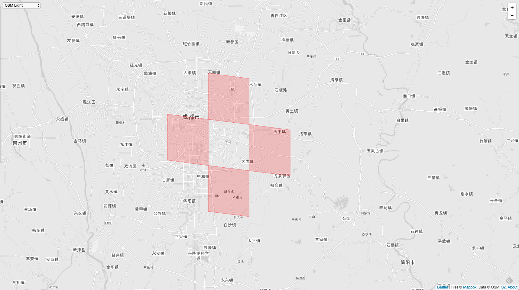
If displayed on a map, it looks like the figure below.
The CellID of the center cell is 3958610196388904960, at Level 10. The edge neighbors computed using the method above are:
3958603599319138304 // bottom neighbor
3958607997365649408 // right neighbor
3958612395412160512 // top neighbor
3958599201272627200 // left neighbor
Displayed on the map:
II. Vertex-Sharing Neighbors
The vertex-sharing neighbors here are slightly different from the vertex neighbors discussed at the beginning of the article. There will also be some seemingly odd examples below—pitfalls I ran into during actual implementation—so I’ll share them here.
First, let’s explain a special case: when a Cell lies exactly on one of the 8 vertices of the cube circumscribing the Earth. In that case, the Cell has only 3 vertex neighbors, not 4. This is because each of those 8 vertices is connected to only 3 faces, so on each face there is exactly one Cell that is its vertex neighbor. Except for Cells at these 8 points, all other Cells have 4 vertex neighbors!
j
|
|  (0,1)  (1,1)
|  (0,0)  (1,0)
|
---------------> i
In the coordinate axes above, if the direction along the i-axis is 1, it falls in the right column of the four quadrants. If the direction along the j-axis is 1, it falls in the top row of the four quadrants.
Assume the Cell Level is not equal to 30; that is, there are still 0s after the trailing marker bit 1. After such a Cell is converted into i and j, the trailing bits of both i and j are 1.
The conclusion above can be proven. In the
faceIJOrientationfunction, when splitting the Cell, if it encounters the all-zero case—for example,orientation = 11and the trailing bits of the Cell are all 0—then it takes the last 8 bits plus the orientation,00000000 11, and after conversion vialookupIJ, obtains1111111111. Thusi = 1111,j = 1111, and the orientation is still11. The trailing00of the Cell continues through the same process, so the trailing bits of i and j all become1111.
Therefore, we only need to determine, based on i and j, which quadrant the Level provided by the input argument falls into, and then we can find all vertex-sharing neighbors.
Assume the Level provided by the input argument is small, meaning the Cell has a large area. In that case, we need to determine which of the four vertices of the input Cell the shared vertex of the current Cell (the function caller) lies on. A Cell is a rectangle with four vertices. Whichever vertex the current Cell (the function caller) is closest to is chosen as the shared vertex. Then, compute the four Cells around that shared vertex in order.
Assume the Level provided by the input argument is large, meaning the Cell has a small area. In that case, we also need to determine which of the four vertices of the current Cell (the function caller) the shared vertex of the input Cell lies on. A Cell is a rectangle with four vertices. Whichever vertex the input Cell is closest to is chosen as the shared vertex. Then, compute the four Cells around that shared vertex in order.
Because we need to determine which quarter of a Cell it lies in, we need to inspect the positions of its four children. That is, we determine the relative positions of the children at Level - 1.
	halfSize := sizeIJ(level + 1)
	size := halfSize << 1
	f, i, j, _ := ci.faceIJOrientation()

	var isame, jsame bool
	var ioffset, joffset int
Here we need to obtain halfSize; halfSize is actually the size of the child cells of the input Cell.
	if i&halfSize != 0 {
		// Located in the right column, so add one cell to the offset
		ioffset = size
		isame = (i + size) < maxSize
	} else {
		// Located in the left column, so subtract one cell from the offset
		ioffset = -size
		isame = (i - size) >= 0
	}
Here we determine which of the rectangle’s four vertices is closest based on whether the halfSize bit is 1. One thing to note is that i + size must not exceed maxSize; if it does, it is no longer on the same face. Similarly, i - size must not be less than 0; if it is, it is also no longer on the same face.
The logic for the j axis is exactly the same as for i.
	if j&halfSize != 0 {
		// On the upper row, so add one cell to the offset
		joffset = size
		jsame = (j + size) < maxSize
	} else {
		// On the lower row, so subtract one cell from the offset
		joffset = -size
		jsame = (j - size) >= 0
	}
For the final computation result, first compute the input Cell, then compute the Cells on the two axes around it.
	results := []CellID{
		ci.Parent(level),
		cellIDFromFaceIJSame(f, i+ioffset, j, isame).Parent(level),
		cellIDFromFaceIJSame(f, i, j+joffset, jsame).Parent(level),
	}
If both i and j are on the same face, then the shared vertex is definitely not one of the 8 vertices of the circumscribed cube. In that case, the Cell of the fourth shared vertex can be computed as well.
	if isame || jsame {
		results = append(results, cellIDFromFaceIJSame(f, i+ioffset, j+joffset, isame && jsame).Parent(level))
	}
In summary, the complete code implementation for computing common vertex neighbors is as follows:
func (ci CellID) VertexNeighbors(level int) []CellID {
	halfSize := sizeIJ(level + 1)
	size := halfSize << 1
	f, i, j, _ := ci.faceIJOrientation()

	fmt.Printf("halfsize original value = %v-%b\n", halfSize, halfSize)
	var isame, jsame bool
	var ioffset, joffset int

	if i&halfSize != 0 {
		// In the back column, so add one cell to the offset
		ioffset = size
		isame = (i + size) < maxSize
	} else {
		// In the left column, so subtract one cell from the offset
		ioffset = -size
		isame = (i - size) >= 0
	}
	if j&halfSize != 0 {
		// In the top row, so add one cell to the offset
		joffset = size
		jsame = (j + size) < maxSize
	} else {
		// In the bottom row, so subtract one cell from the offset
		joffset = -size
		jsame = (j - size) >= 0
	}

	results := []CellID{
		ci.Parent(level),
		cellIDFromFaceIJSame(f, i+ioffset, j, isame).Parent(level),
		cellIDFromFaceIJSame(f, i, j+joffset, jsame).Parent(level),
	}

	if isame || jsame {
		results = append(results, cellIDFromFaceIJSame(f, i+ioffset, j+joffset, isame && jsame).Parent(level))
	}

	return results
}
Let’s look at a few examples.
The first example uses Cells of the same size. Both the input argument and the caller Cell are at the same Level - 10.
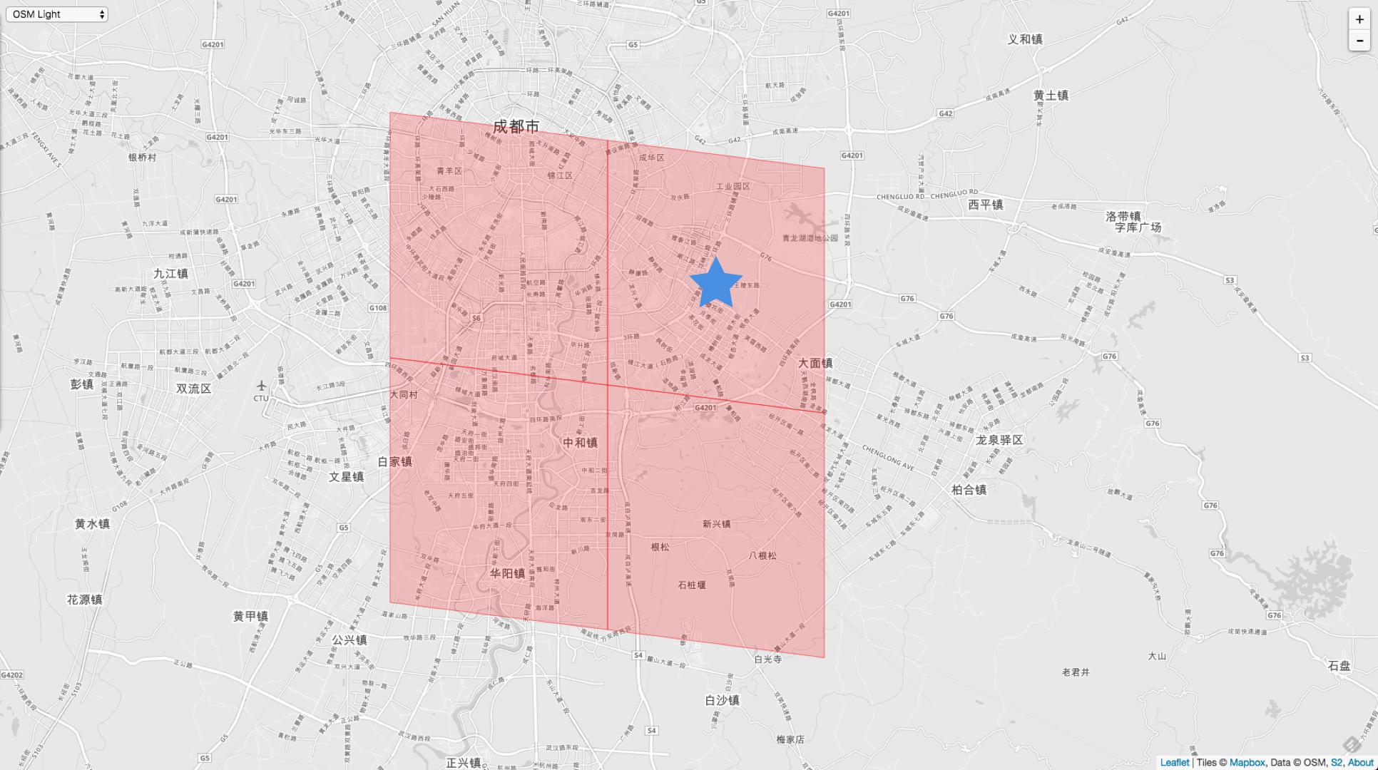
VertexNeighbors := cellID.Parent(10).VertexNeighbors(10)

// 11011011101111110011110000000000000000000000000000000000000000
3958610196388904960 // upper right corner
3958599201272627200 // upper left corner
3958603599319138304 // lower right corner
3958601400295882752 // lower left corner
Is the second example a Cell of a different size? The calling Cell is at the default Level - 30.
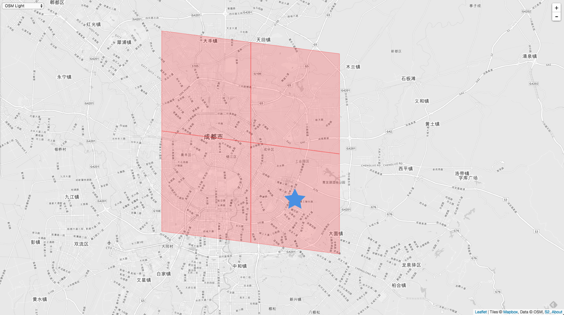
VertexNeighbors := cellID.VertexNeighbors(10)

// 11011011101111110011110000000000000000000000000000000000000000
3958610196388904960 // lower right corner
3958599201272627200 // lower left corner
3958612395412160512 // upper right corner
3958623390528438272 // upper left corner
The two examples above illustrate an issue: even though the Cells returned by calling VertexNeighbors(10) are all at Level 10, their orientations and positions differ. Fundamentally, the vertex they share is different, so the generation directions of the four resulting Cells are also different.
In the C++ version, finding vertex neighbors has one limitation:
DCHECK_LT(level, this->level());
The input Level must be strictly lower than the Level of the Cell being searched for. In other words, the grid area of the input Cell must be smaller than the Cell’s grid size. However, the Go implementation does not have this requirement; the input can be either larger or smaller.
In the example below, the input has a lower Level than the Cell. (You can see that Chengdu has already become as small as a single point.)
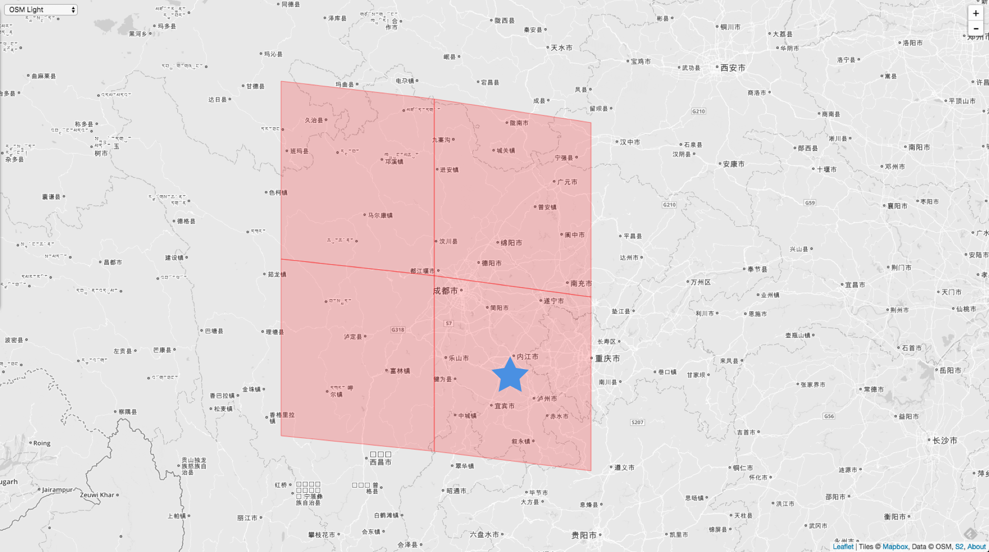
VertexNeighbors := cellID.Parent(10).VertexNeighbors(5)

3957538172551823360 // lower right corner
3955286372738138112 // lower left corner
3959789972365508608 // upper right corner
3962041772179193856 // upper left corner
In the example below, the input argument is greater than the Cell’s Level. (You can see that the area at Level 15 is already very small.)
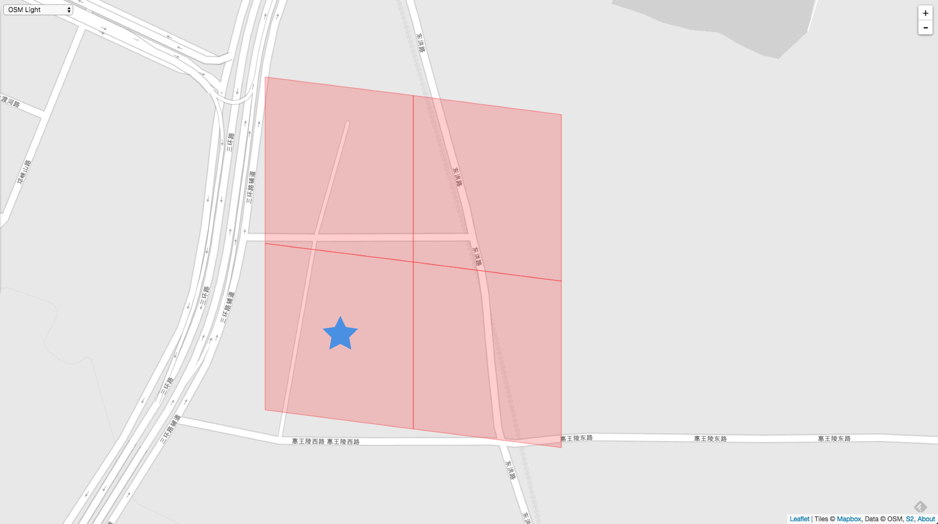
VertexNeighbors := cellID.Parent(10).VertexNeighbors(15)


3958610197462646784 // lower-left corner
3958610195315163136 // lower-right corner
3958610929754570752 // upper-left corner
3958609463023239168 // upper-right corner
III. All Neighbors
Finally, let’s return to the question raised at the beginning of the article: how do we find the neighbors of a Hilbert curve on a quadtree? With the groundwork laid above, the answer may already be clear to the reader.
Finding all neighbors has one requirement: the area represented by the input Level must be smaller than or equal to that of the caller Cell. In other words, the input Level value must not be smaller than the caller’s Level. If it were smaller, the neighboring Cell would cover a much larger area, and a single neighboring Cell could very likely contain all of the original Cell’s neighbors. Such a lookup would be meaningless.
For example, if the input Level is smaller than the caller Cell’s Level, then when finding all of its neighbors, the result would look like this:
AllNeighbors := cellID.Parent(10).AllNeighbors(5)
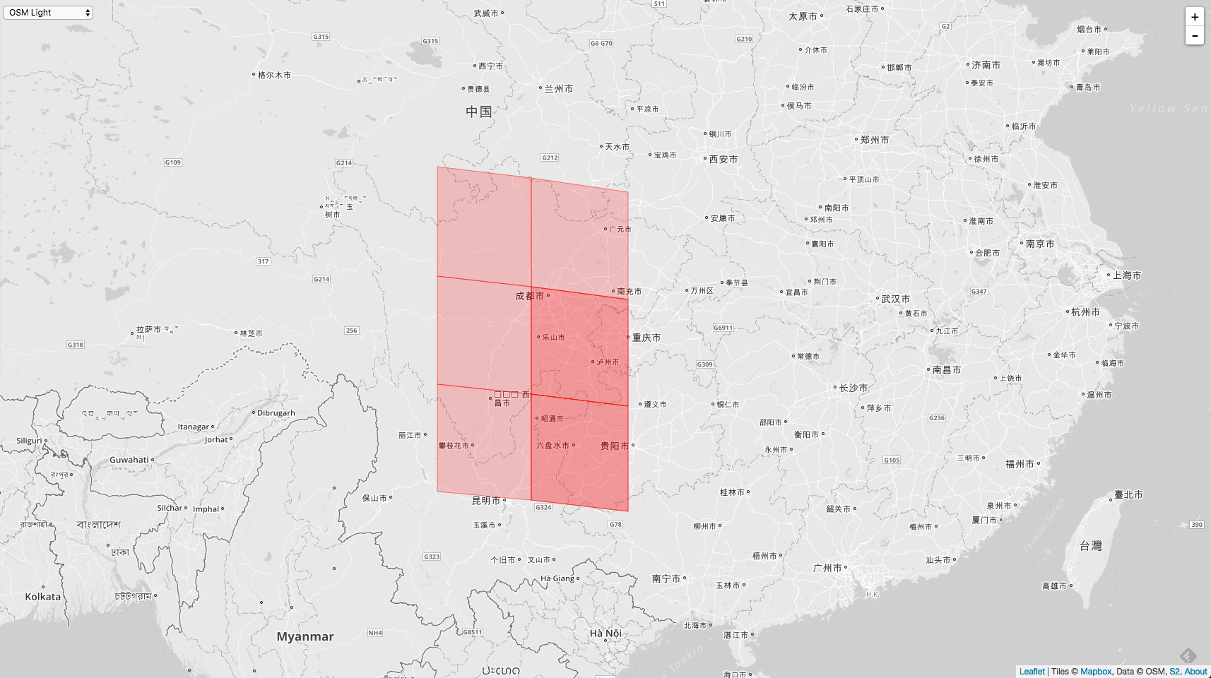
At this point, all neighbors can be found, but overlapping Cells may occur. Why this happens will be analyzed below.
If the input parameter and the caller Cell have the same Level, then the full set of neighbors found is exactly the problem described at the beginning of the article. The ideal case is as follows:
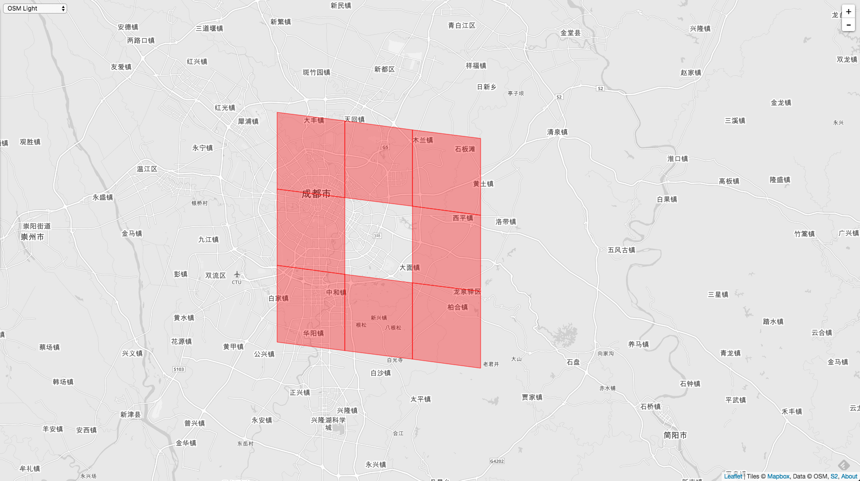
The concrete implementation is as follows:
func (ci CellID) AllNeighbors(level int) []CellID {
	var neighbors []CellID

	face, i, j, _ := ci.faceIJOrientation()

	// Find the coordinates of the bottom-leftmost leaf node. We need to normalize the i, j coordinates, because the input Level may be greater than the caller Cell's Level.
	size := sizeIJ(ci.Level())
	i &= -size
	j &= -size

	nbrSize := sizeIJ(level)

	for k := -nbrSize; ; k += nbrSize {
		var sameFace bool
		if k < 0 {
			sameFace = (j+k >= 0)
		} else if k >= size {
			sameFace = (j+k < maxSize)
		} else {
			sameFace = true
			// Upper and lower neighbors
			neighbors = append(neighbors, cellIDFromFaceIJSame(face, i+k, j-nbrSize,
				j-size >= 0).Parent(level))
			neighbors = append(neighbors, cellIDFromFaceIJSame(face, i+k, j+size,
				j+size < maxSize).Parent(level))
		}

		// Left and right neighbors, plus the two diagonal vertex neighbors
		neighbors = append(neighbors, cellIDFromFaceIJSame(face, i-nbrSize, j+k,
			sameFace && i-size >= 0).Parent(level))
		neighbors = append(neighbors, cellIDFromFaceIJSame(face, i+size, j+k,
			sameFace && i+size < maxSize).Parent(level))

		// This condition has two purposes: prevent 32-bit overflow, and serve as the loop exit condition; once k exceeds size, there is no need to keep looking.
		if k >= size {
			break
		}
	}

	return neighbors
}
The general idea of the code above has been described in the comments. The parts that need further explanation are covered below.
The first thing to understand is the relationship between nbrSize and size. Why do we need nbrSize? Because the input Level can be different from the caller Cell's Level. The Cell represented by the input Level may be larger, smaller, or the same size. The final result is expressed in terms of grid cells of size nbrSize, so the loop needs to use nbrSize to control the grid cell size. size, on the other hand, is only the grid cell size of the original caller Cell.
Now look at how k changes in the loop. When k = -nbrSize, the loop only computes the left and right neighbors. The vertex neighbors on the diagonals are actually special cases of the left and right neighbors. Next, when k = 0, it starts computing the top and bottom neighbors. k keeps increasing until eventually k >= size; in the final iteration, it computes the left and right neighbors once more, then exits via break.
The caller Cell is in the middle, so to skip over this Cell and reach the other side—either vertically or horizontally—you need to skip by size. In the code, this is implemented as i + size and j + size.
First, look at how the left and right neighbors are scanned.
The left neighbor is i - nbrSize, j + k, with k changing in the loop. This is how the left neighbors are generated. It generates a column of left neighbors, starting from the lower-left corner and continuing upward to the upper-left corner.
The right neighbor is i + size, j + k, with k changing in the loop. This is how the right neighbors are generated. It generates a column of right neighbors, starting from the lower-right corner and continuing upward to the upper-right corner.
Now look at how the top and bottom neighbors are scanned.
The bottom neighbor is i + k, j - nbrSize, with k changing in the loop. This is how the bottom neighbors are generated. It generates a row of bottom neighbors, starting from the leftmost bottom neighbor and continuing to the rightmost bottom neighbor.
The top neighbor is i + k, j + size, with k changing in the loop. This is how the top neighbors are generated. It generates a row of top neighbors, starting from the leftmost top neighbor and continuing to the rightmost top neighbor.
Example:
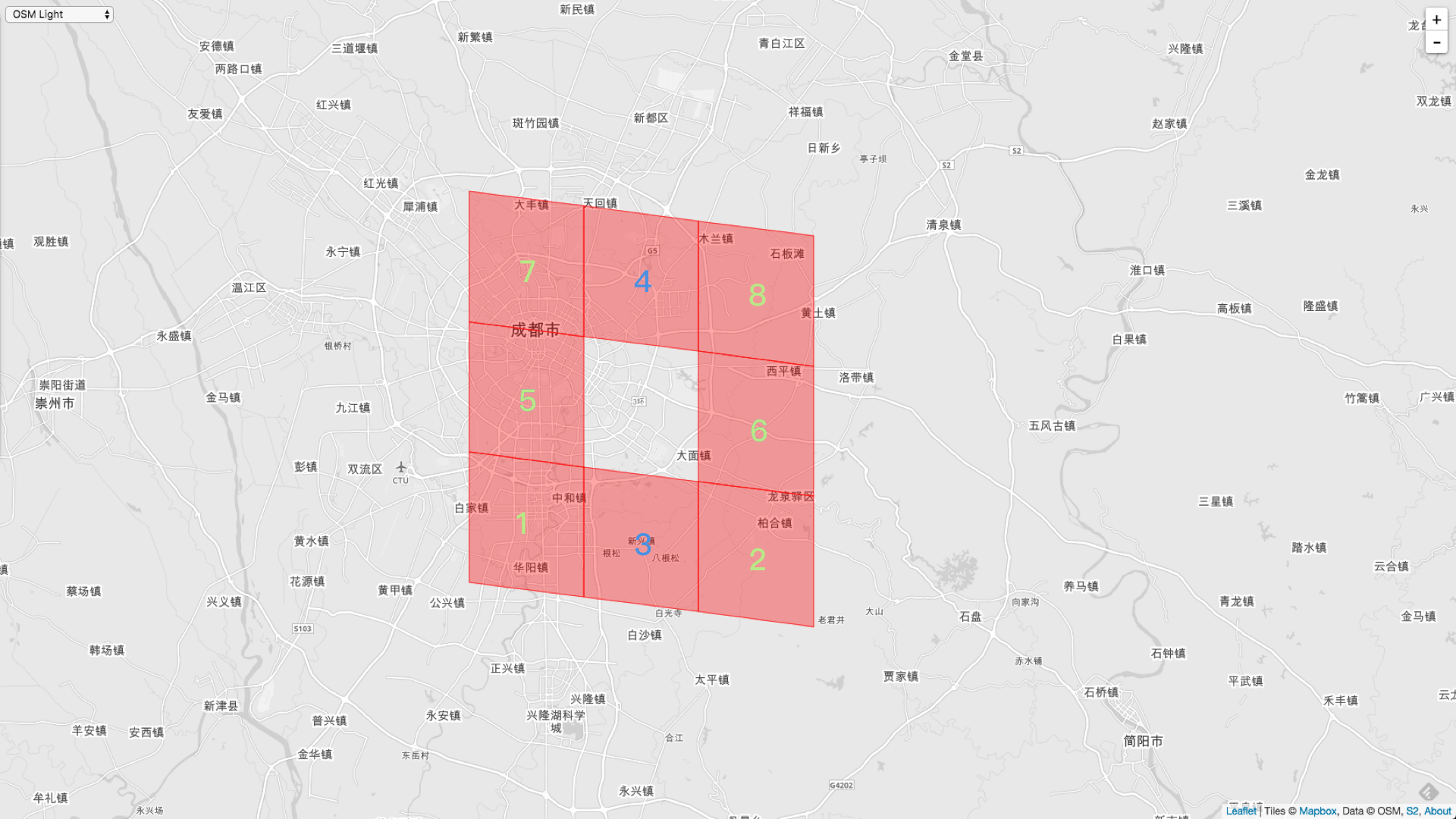
The full set of neighbors around the middle Cell consists of the eight Cells at the same Level shown in the figure above.
The generation order is labeled in the figure. 1, 2, 5, 6, 7, and 8 are generated as left and right neighbors. 3 and 4 are generated as top and bottom neighbors.
In the example above, all Cells are generated at Level - 10. The full neighbor set happens to contain exactly eight Cells.
AllNeighbors := cellID.Parent(10).AllNeighbors(10)

3958601400295882752,
3958605798342393856,
3958603599319138304,
3958612395412160512,
3958599201272627200,
3958607997365649408,
3958623390528438272,
3958614594435416064
Here’s another example where the Level is greater than the caller Cell’s Level.
AllNeighbors := cellID.Parent(10).AllNeighbors(11)

3958600575662161920,
3958606622976114688,
3958603324441231360,
3958611570778439680,
3958600025906348032,
3958607172731928576,
3958603874197045248,
3958613220045881344,
3958599476150534144,
3958608821999370240,
3958623115650531328,
3958613769801695232
Its full-neighbor generation order is as follows:
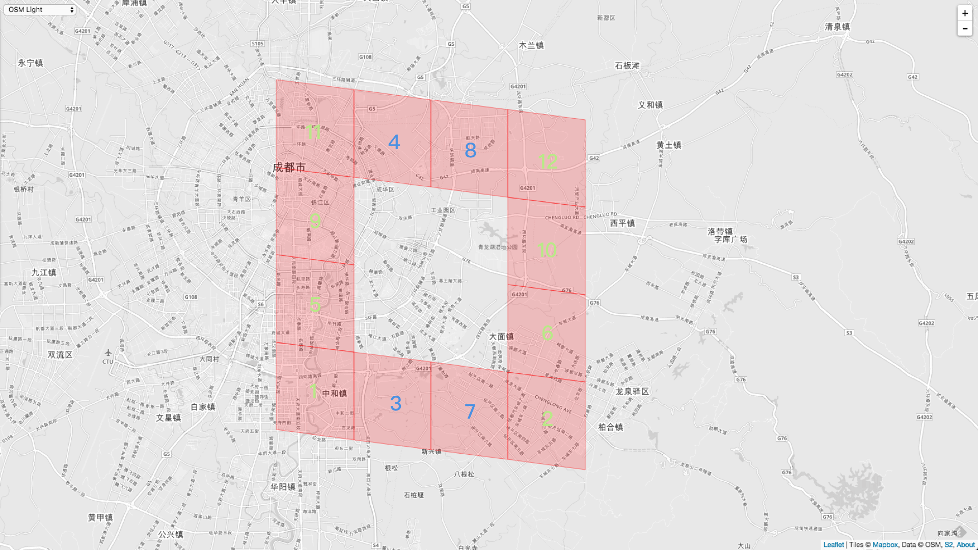
1, 2, 5, 6, 9, 10, 11, and 12 are left/right neighbors, while 3, 4, 7, and 8 are top/bottom neighbors. We can see that left/right neighbors are generated from bottom to top, and top/bottom neighbors are generated from left to right.
If the Level is larger, for example Level - 15, more neighbors will be generated:
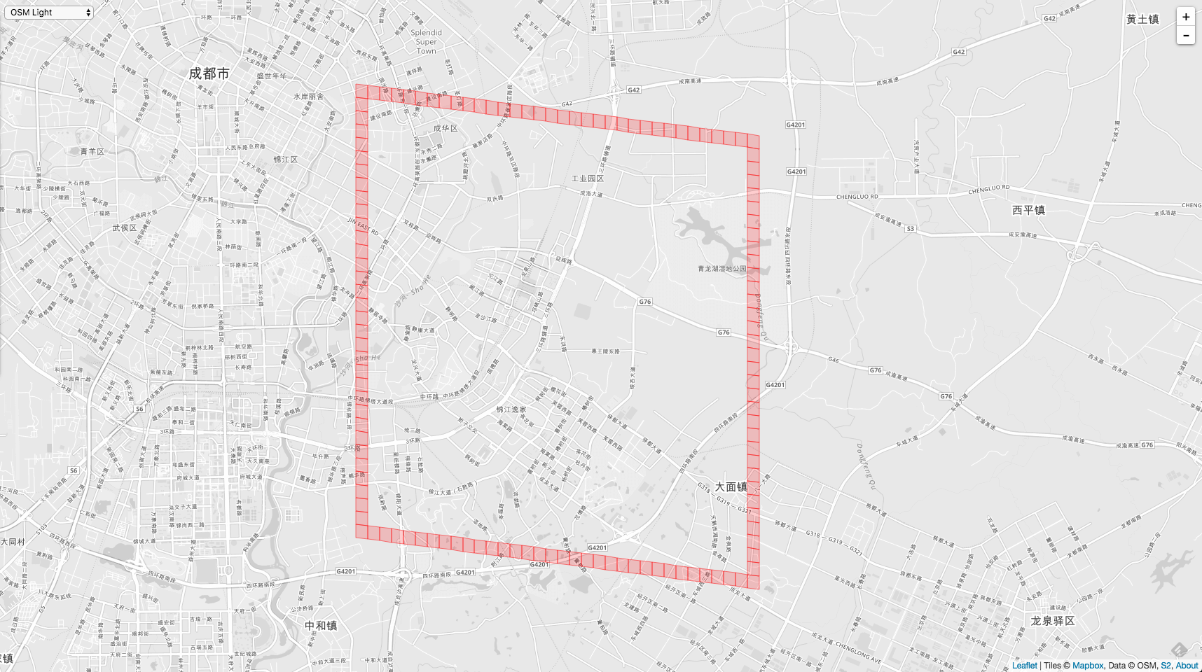
Now let’s explain the case where the input Level is smaller than the Level of the caller Cell.
For example, input Level = 9.
AllNeighbors := cellID.Parent(10).AllNeighbors(9)

3958589305667977216,
3958580509574955008,
3958580509574955008,
3958615693947043840,
3958598101760999424,
3958606897854021632,
3958624490040066048,
3958615693947043840
The generated full set of neighbors is as follows:
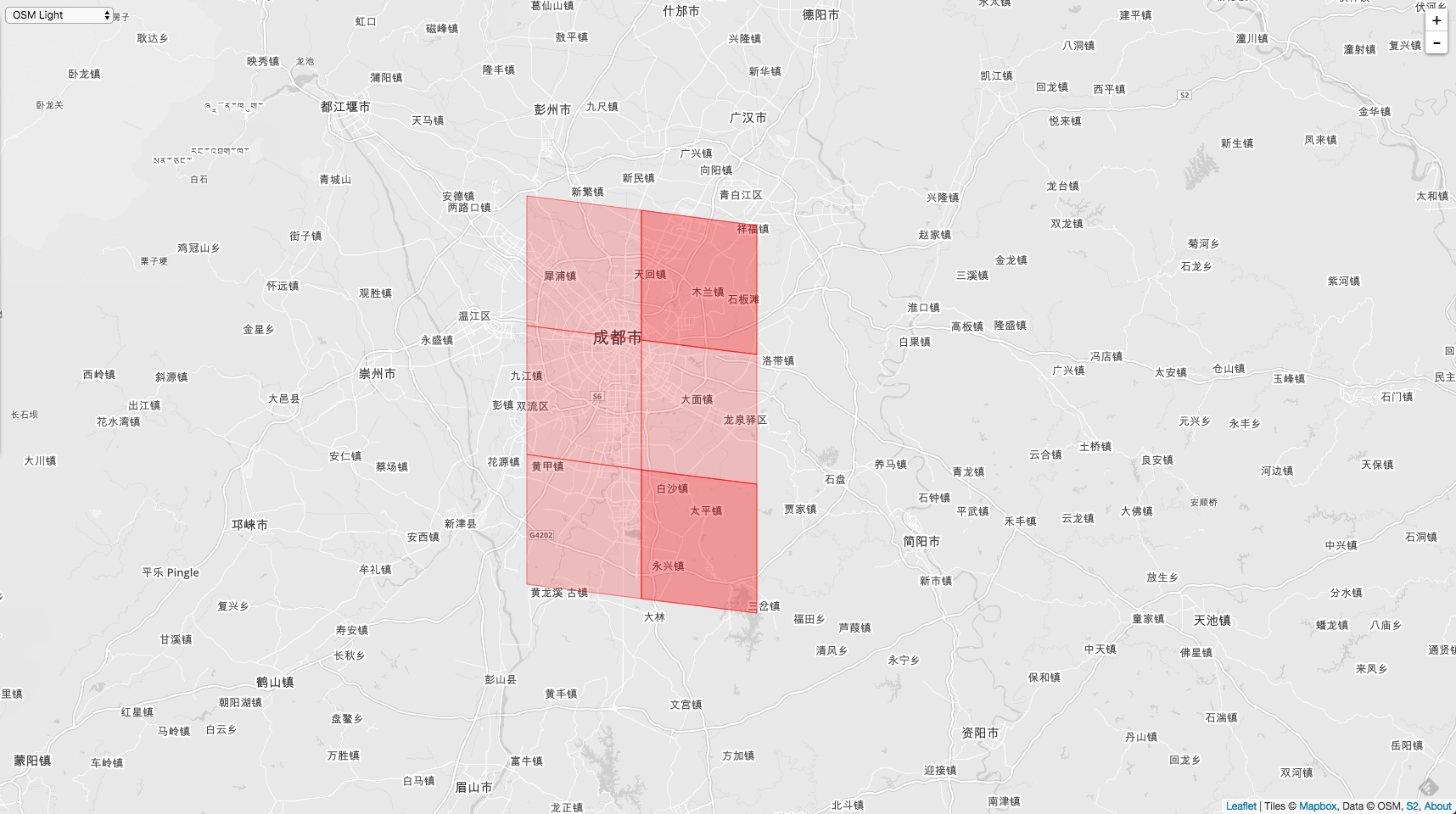
As you can see, there were originally 8 neighbors, but now there are only 6. In fact, 8 were still generated; it is just that 2 of them are duplicates. The duplicates are the two dark red Cells in the figure.
Why do they overlap?
The caller’s intermediate Level - 10 Cell is drawn first.
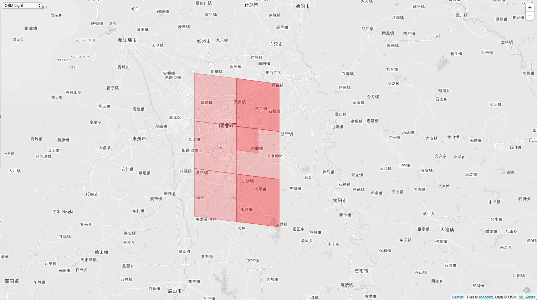
Because it is Level - 9, it is one quarter of the Cell in the middle.
Now let’s also draw the two upper neighbors of the Level - 10 Cell.
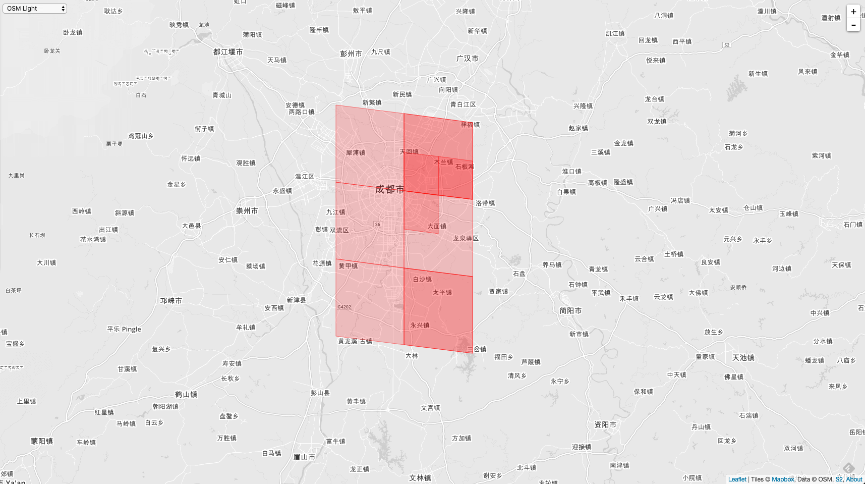
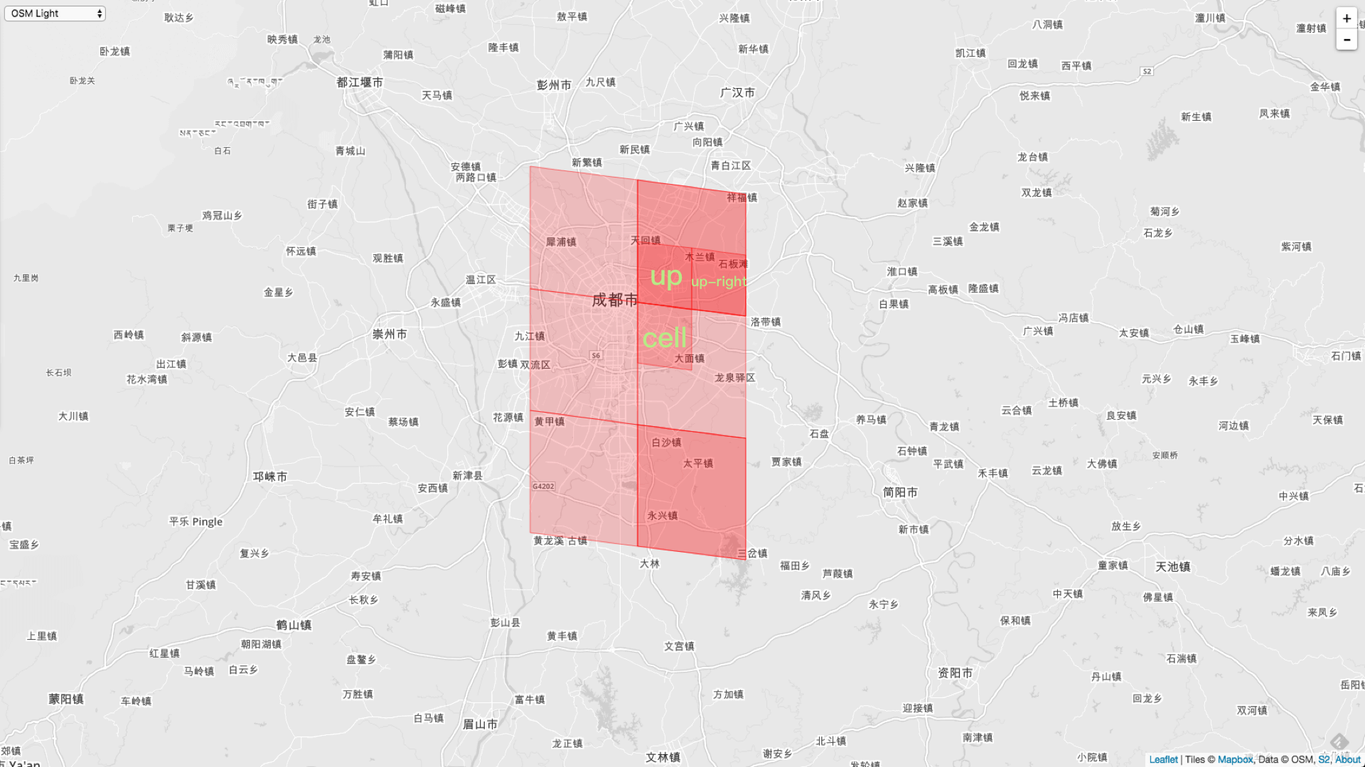
As you can see, the upper neighbor Up and the vertex neighbor up-right are both located within the same Level - 9 Cell. Therefore, the upper neighbor and the upper-right vertex neighbor are both the same Level - 9 Cell, so they overlap. Similarly, the lower neighbor and the lower-right vertex neighbor also overlap. As a result, 2 Cells overlap.
Also, the caller Cell’s position is not left empty in the middle. This is because after i + size, the range is still within the same Level - 9 Cell.
If the Level is smaller, the overlap pattern changes again. For example, Level - 5.
AllNeighbors := cellID.Parent(10).AllNeighbors(5)

3953034572924452864,
3946279173483397120,
3946279173483397120,
3957538172551823360,
3955286372738138112,
3957538172551823360,
3962041772179193856,
3959789972365508608
Drawn on a map, it looks like this:
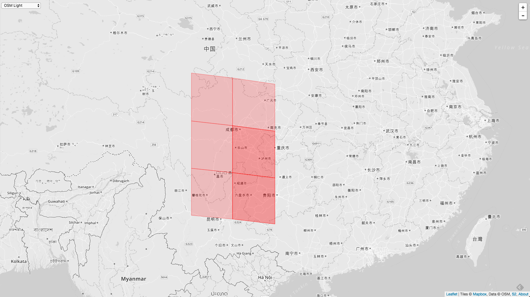
The overlapping positions have also changed.
At this point, all algorithms related to finding neighbors have been covered.
Articles in the Spatial Search series:
How to Understand n-Dimensional Space and n-Dimensional Spacetime
Efficient Multidimensional Spatial Point Indexing Algorithms — Geohash and Google S2
How Is CellID Generated in Google S2?
Finding the LCA (Lowest Common Ancestor) in a Quadtree in Google S2
The Magical De Bruijn Sequence
How to Find Hilbert Curve Neighbors on a Quadtree?
GitHub Repo: Halfrost-Field
Follow: halfrost · GitHub