Finding the LCA (Lowest Common Ancestor) in Google S2 Quadtrees
I. Finding Parent Nodes and Child Nodes
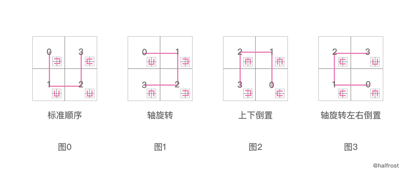
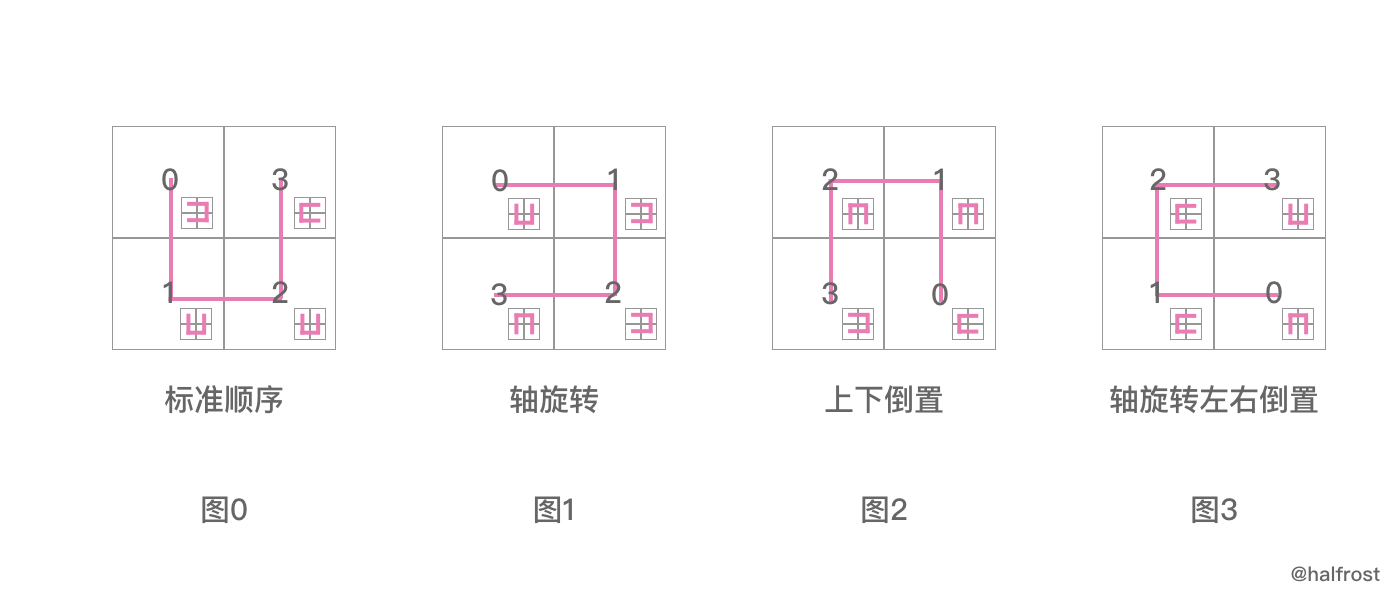
First, we need to review how Hilbert curves are generated. For the specific code, see the analysis in the author’s previous article. In that analysis, four directions are particularly important and are needed for the following discussion, so the diagrams for these four directions are included here.
Before giving examples, one more point needs to be clarified. Some websites provide binary conversion without indicating whether the conversion is signed or unsigned, which can lead to misunderstandings. The author did not notice this issue at first and fell into this trap; it took quite a while to realize what was going on. After checking many online conversion calculators, the author found this issue in all of them. For example, with the commonly used online base converter http://tool.oschina.net/hexconvert, if you pick any two 64-bit binary numbers and convert the signed and unsigned versions to decimal respectively—or convert them back the other way—you will be pleasantly surprised to find that the two results are actually the same! For example, if you enter 3932700003016900608 and 3932700003016900600, you will find that after conversion to binary, both results are 11011010010011110000011101000100000000000000000000000000000000. But clearly, these two numbers are different.
If 3932700003016900608 is unsigned and 3932700003016900600 is signed, the correct results should be as follows:
// 3932700003016900608
11011010010011110000011101000100000000000000000000000000000000

// 3932700003016900600
11011010010011110000011101000011111111111111111111111111111000
The gap is clearly quite large. There are actually many examples like this; here are a few more at random: unsigned 3932700011606835200 and signed 3932700011606835000; unsigned 3932700020196769792 and signed 3932700020196770000; unsigned 3932700028786704384 and signed 3932700028786704400… There are many more examples, so I won’t list them all here.
With this online tool, decimal-to-binary conversion is unsigned, while binary-to-decimal conversion becomes signed. However, Google S2 uses unsigned CellIDs by default, so using signed CellIDs will lead to errors. You need to be careful about this during conversion. I ran into some issues before noticing this; once I suddenly realized it, everything became clear.
All right, let’s get to the main topic. Next, let’s look directly at an example. I’ll use it to explain the relationships between Cells and how to find a parent node.
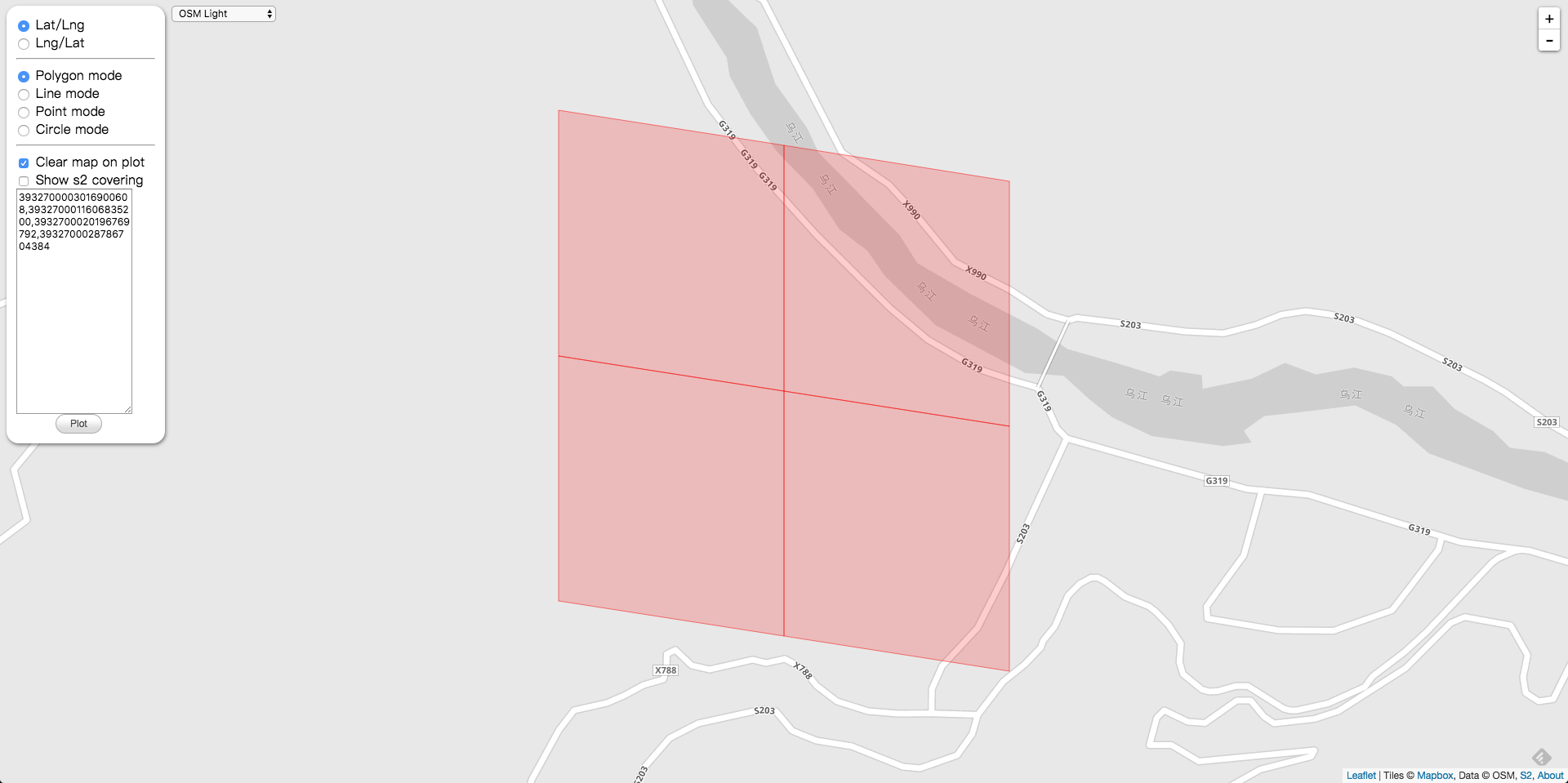
Assume there are four connected Cells as shown above. First, compute the CellID from the latitude and longitude.
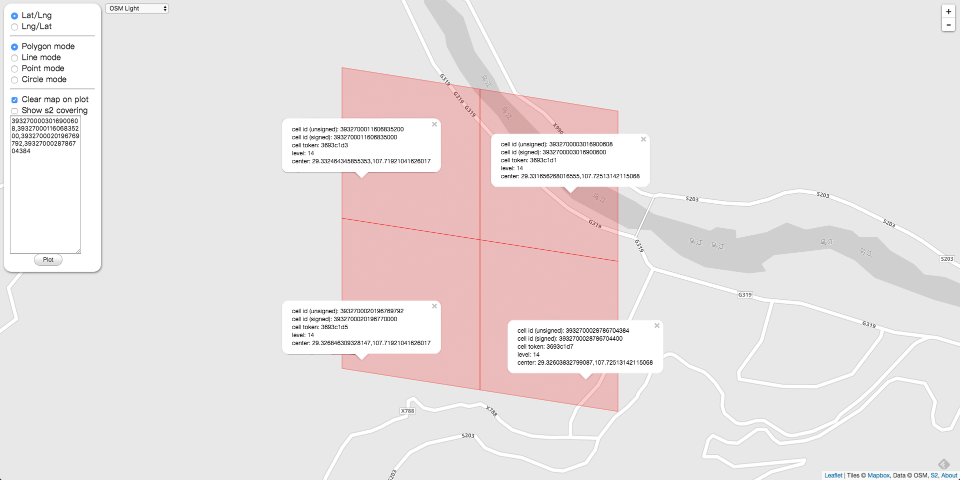
The corresponding four CellIDs are:
Since the first two bits are both 0, they could actually be omitted, but for clarity, I still filled it out to 64 bits and kept the leading two 0s.

// 3932700003016900608 upper right
0011011010010011110000011101000100000000000000000000000000000000

// 3932700011606835200 upper left
0011011010010011110000011101001100000000000000000000000000000000

// 3932700020196769792 lower left
0011011010010011110000011101010100000000000000000000000000000000

// 3932700028786704384 lower right
0011011010010011110000011101011100000000000000000000000000000000
In the previous article, we also analyzed the 64-bit structure of a Cell. Here we have four Level 14 Cells, so there are 64 - 3 - 1 - 14 * 2 = 32 trailing 0s. The 33rd bit from the end is a 1, and the 34th and 35th bits are what we need to focus on. As you can see, they are 00, 01, 10, and 11, respectively—exactly four consecutive binary values.
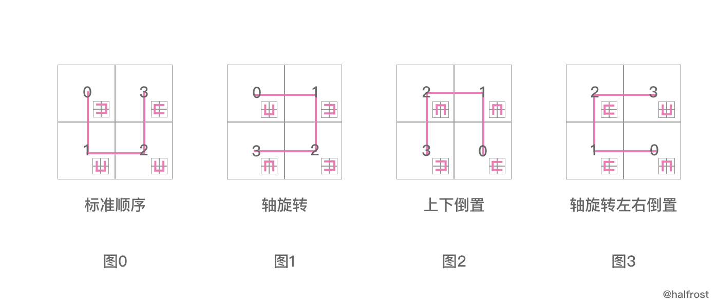
Based on this order, we can match the order of these four current Level 14 Cells to Figure 0 in the diagram above. The only difference is that the current orientation is rotated by about 45°.
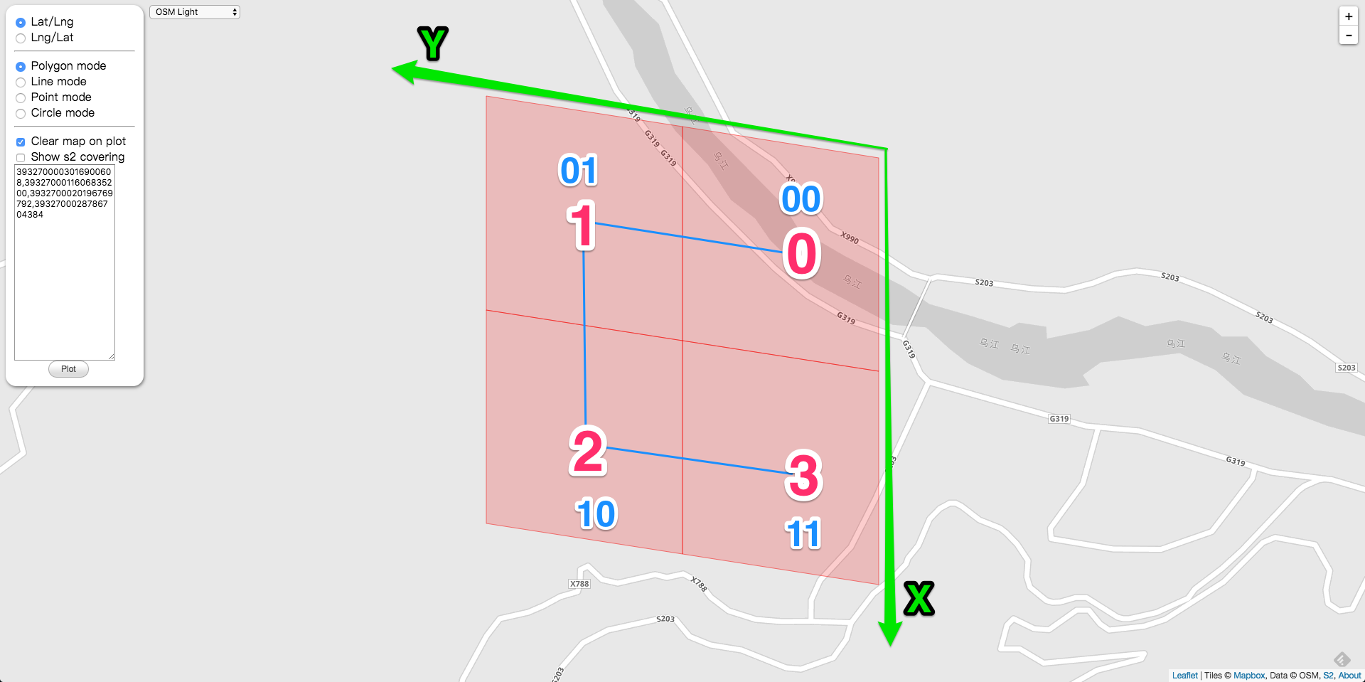
The CellID in the upper right is 3932700003016900608. The 34th and 35th bits from right to left are 00. Starting from this upper-right Cell, if we want to find the next Cell on the Hilbert curve, since its current orientation is the orientation shown in Figure 0, the next Cell after the upper-right Cell is the upper-left Cell. Therefore, the 34th and 35th bits should be 01. After changing them to 01, we get 3932700011606835200, which is the corresponding CellID. The 34th bit from the right has increased by 1, which corresponds to an increase of 2^33^ = 8589934592 in decimal. If we compute the decimal difference between the two CellIDs, it is exactly this value. So far, everything is correct.
By the same reasoning, the next Cell after the upper-left Cell is the lower-left Cell. Again, the 34th and 35th bits become 10, corresponding to an increase of 2^33^ = 8589934592 in decimal, giving the lower-left CellID as 3932700020196769792. Continuing in the same way, we can obtain the last CellID, the lower-right CellID, which is 3932700028786704384.
At this point, readers should have a very clear understanding of how to find sibling nodes at the same Level. Some may wonder: what does finding parent and child nodes have to do with siblings? The connection lies in the four orientation diagrams mentioned at the beginning of this section.
Recall how the Hilbert curve is generated. During the recursive generation of the Hilbert curve, a posToIJ array is maintained, and this array records the four orientations. The way the Hilbert curve is generated is closely tied to these four orientations. If you have forgotten this part, please refer back to the author’s analysis article.
So, when looking for child nodes at the same Level, we first need to determine the current Cell’s position within that Level and which of the four orientations the current Cell is in. This orientation determines the position of the child to be found at the next Level, or at some deeper Level. The Hilbert curve is effectively a quadtree: each root node has four children. Although it is easy to traverse by level to reach the level where the child resides, a single root node has four children, and deciding which one to choose requires judging the parent node’s orientation level by level.
Here is an example to illustrate this issue:
func testS2() {

	latlng := s2.LatLngFromDegrees(29.323773, 107.727194)
	cellID := s2.CellIDFromLatLng(latlng)
	cell := s2.CellFromCellID(cellID) //9279882742634381312

	// cell.Level()
	fmt.Println("latlng = ", latlng)
	fmt.Println("cell level = ", cellID.Level())
	fmt.Printf("cell = %d %b\n", cellID, cellID)
	smallCell := s2.CellFromCellID(cellID.Parent(13))
	fmt.Printf("smallCell level = %d\n", smallCell.Level())
	fmt.Printf("smallCell id = %d / cellID = %d /smallCell(14).Parent = %d (level = %d)/smallCell(15).Parent = %d (level = %d)/cellID(13).Parent = %d (level = %d)/cellID(14).Parent = %d (level = %d)/cellID(15).Parent = %d (level = %d)/ %b \n", smallCell.ID(), cellID, smallCell.ID().Parent(14), (smallCell.ID().Parent(14).Level()), smallCell.ID().Parent(15), (smallCell.ID().Parent(15).Level()), cellID.Parent(13), (cellID.Parent(13)).Level(), cellID.Parent(14), (cellID.Parent(14)).Level(), cellID.Parent(15), (cellID.Parent(15)).Level(), smallCell.ID())

}
Consider what the program above would output. Or, to put it another way: for the same node, if we first find its Level 13 ancestor, and then from that Level 13 node find its Level 15 ancestor, will the resulting Level 15 node be the same as if we directly found its Level 15 ancestor?
Of course, finding Level 13 first and then Level 15 does not produce Level 28. This is not an additive relationship; the result is still the Level 15 ancestor. So both approaches produce a Level 15 node. But are the results obtained by the two approaches the same? You can take a guess first.
The actual result is as follows:
latlng =  [29.3237730, 107.7271940]
cell level =  30
cell = 3932700032807325499 11011010010011110000011101011111101111101001011100111100111011
smallCell level = 13
smallCell id = 3932700015901802496 / cellID = 3932700032807325499 /smallCell(14).Parent = 3932700020196769792 (level = 14)/smallCell(15).Parent = 3932700016975544320 (level = 15)/cellID(13).Parent = 3932700015901802496 (level = 13)/cellID(14).Parent = 3932700028786704384 (level = 14)/cellID(15).Parent = 3932700032007929856 (level = 15)/ 11011010010011110000011101010000000000000000000000000000000000
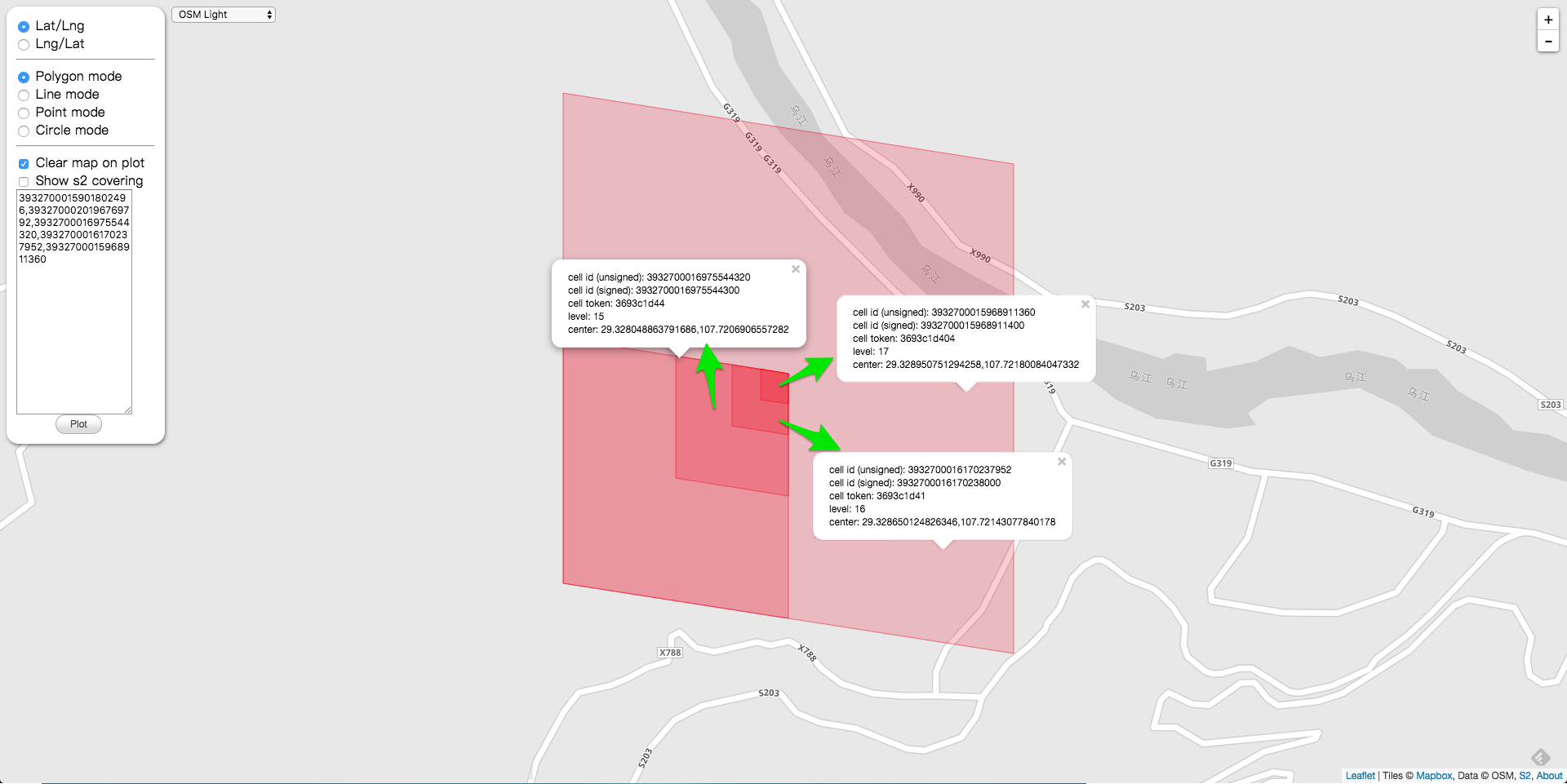
As you can see, the results produced by the two approaches are different. But where exactly do they differ? Looking at the CellID directly is not very intuitive, so let’s draw both of them and take a look.
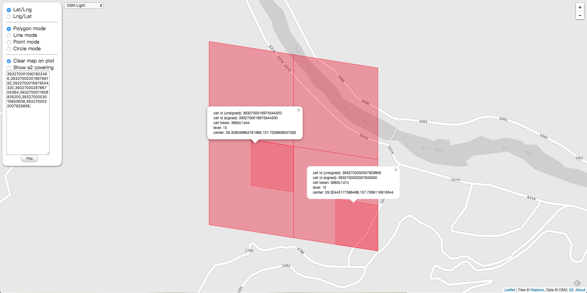
As you can see, although the two have the same Level, their positions are different. Why does this happen? The reason is what we discussed earlier: in a quadtree with four children, which child is selected is determined by the direction of the parent node.
1. Finding Child Nodes
Continuing with the example from the program above, let’s look at how to find child nodes.
We print out all nodes from Level 13 to Level 17.
smallCell id = 3932700015901802496 (level = 13)/
smallCell(14).Parent = 3932700020196769792 (level = 14)/
smallCell(15).Parent = 3932700016975544320 (level = 15)/
smallCell(16).Parent = 3932700016170237952 (level = 16)/
smallCell(17).Parent = 3932700015968911360 (level = 17)/
Drawn on the diagram,
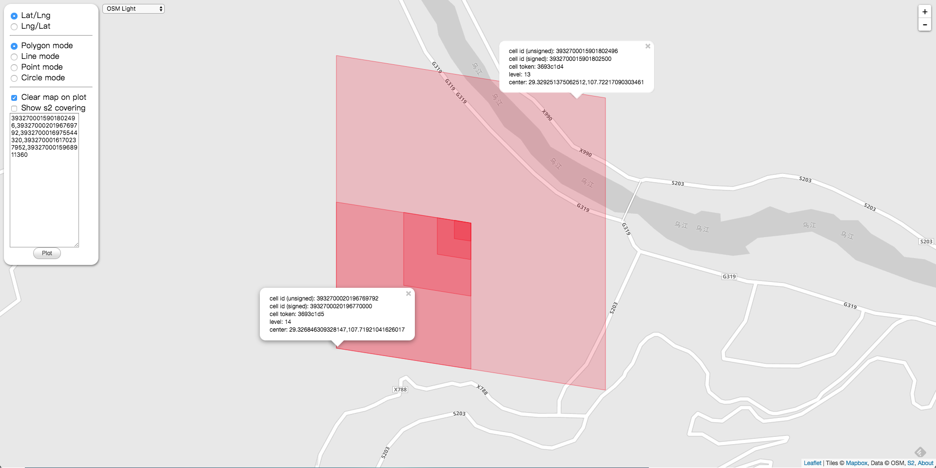
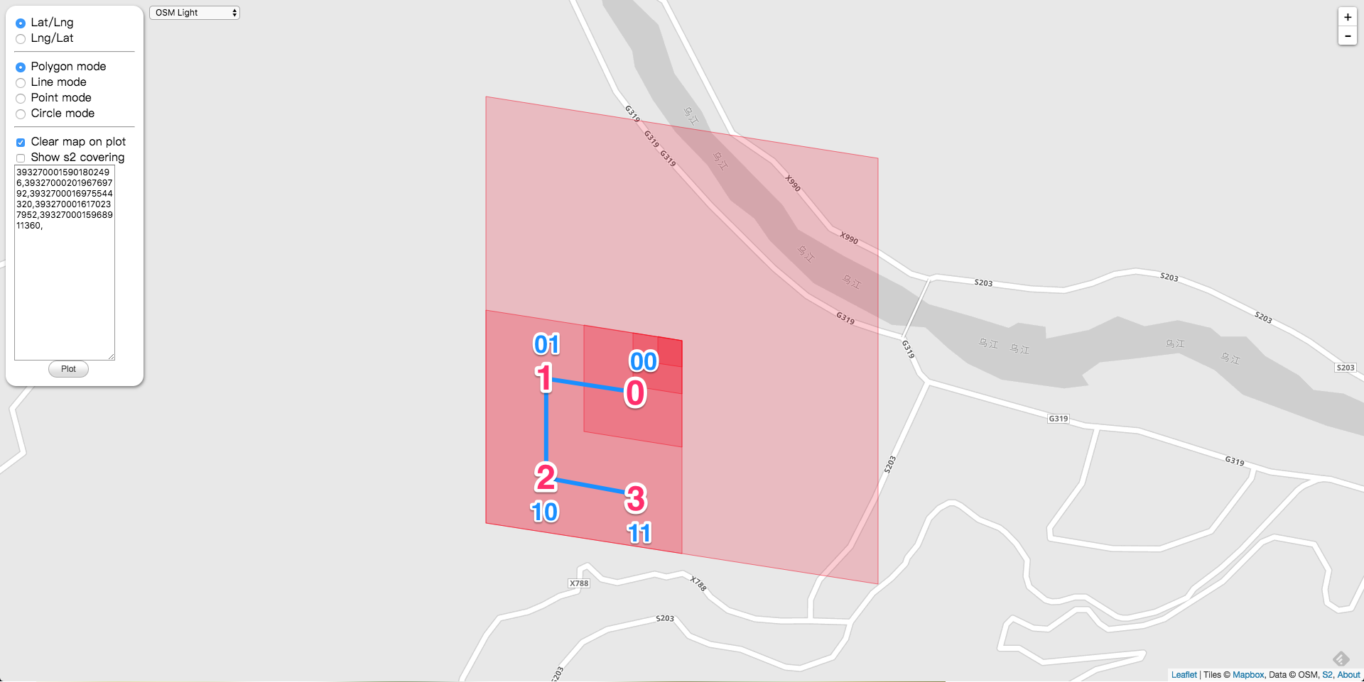
How does Level 13 transform into Level 14? We know the currently selected direction is that of Figure 0. Therefore, the current Level 14 is position 2 in Figure 0.
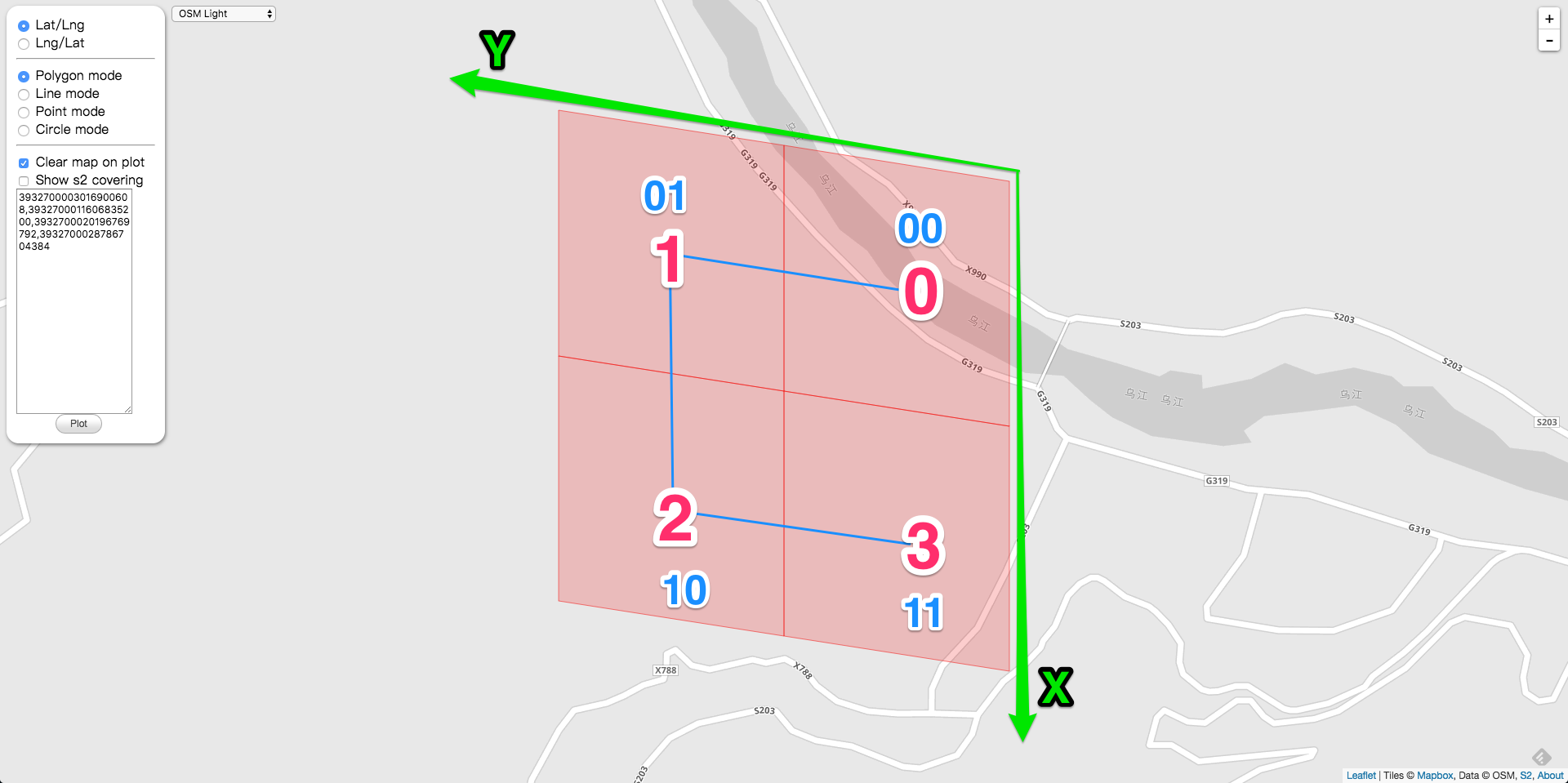
So, counting from right to left, bits 64 - 3 - 1 - 13 * 2 = 34 and 35 should be filled with 01 respectively; read from front to back, that is 10, which corresponds to position 2 in the figure above. Also, the trailing flag bit 1 is moved back by another 2 bits.
11011010010011110000011101010000000000000000000000000000000000   13
11011010010011110000011101010100000000000000000000000000000000   14
This transforms Level 13 to Level 14. This is the method for transforming from a parent node to a child node.
Similarly, let’s look at how Level 15, Level 16, and Level 17 are transformed.
As mentioned earlier, when inspecting a child node, you need to know the directions of the current node’s other three sibling nodes.
According to the figure below, Level 14 corresponds to figure 0, and position 2 is currently selected. From the figure below, you can see that the next-level figure for position 2 in figure 0 is “U”-shaped, which means it still has the shape of figure 0.
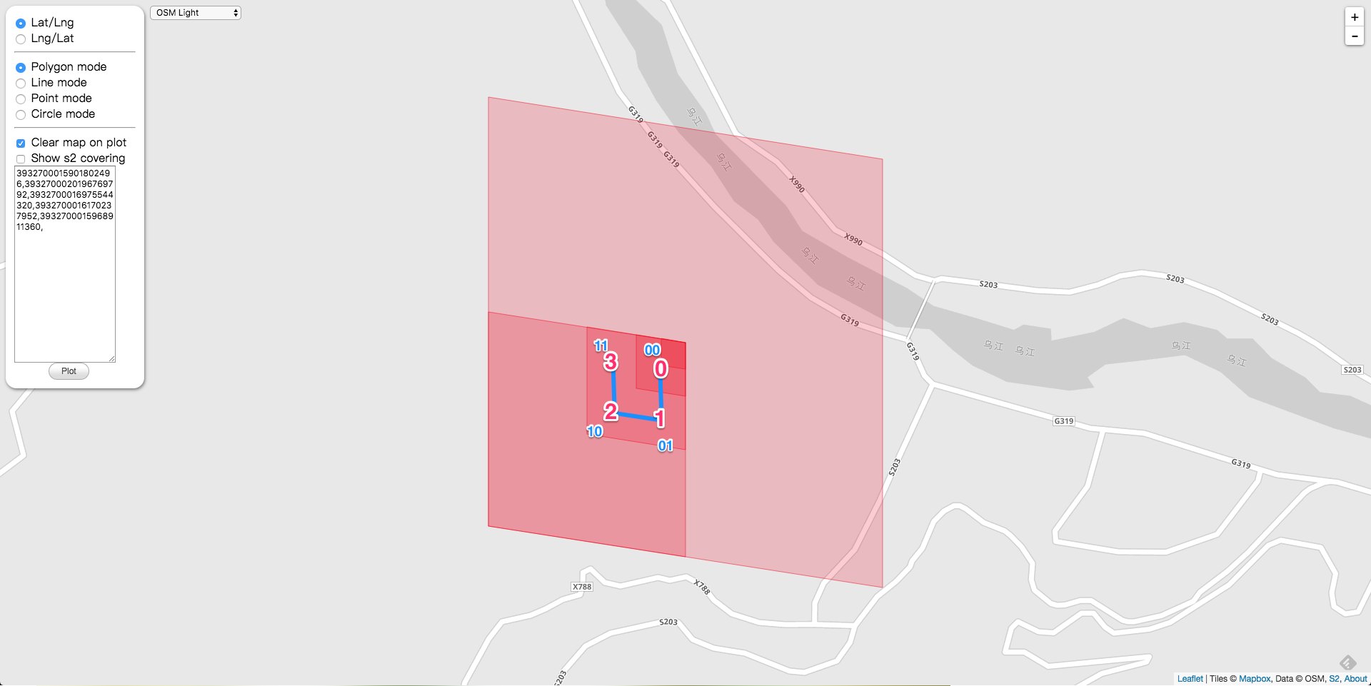
Therefore, we can tell that the current direction at Level 14 is still figure 0. Mark the directions on the figure as shown below.
So if position 0 in the figure above is still selected, then for Level 15, fill in 00 at bits 64 - 3 - 1 - 14 * 2 = 32 and 33, counting from right to left.
11011010010011110000011101010100000000000000000000000000000000   14
11011010010011110000011101010001000000000000000000000000000000   15
Since position 0 in Figure 0 is selected, the direction of the next level corresponds to Figure 1. (Note that the entire diagram is rotated 90° to the left.)
In Figure 1, position 0 is selected again, so in Level 16, counting from right to left, positions 64 - 3 - 1 - 15 * 2 = 30 and 31 are filled with 00. This gives us Level 16.
11011010010011110000011101010001000000000000000000000000000000   15
11011010010011110000011101010000010000000000000000000000000000   16
Because position 0 in Figure 1 is selected, the direction for the next level still corresponds to Figure 0.
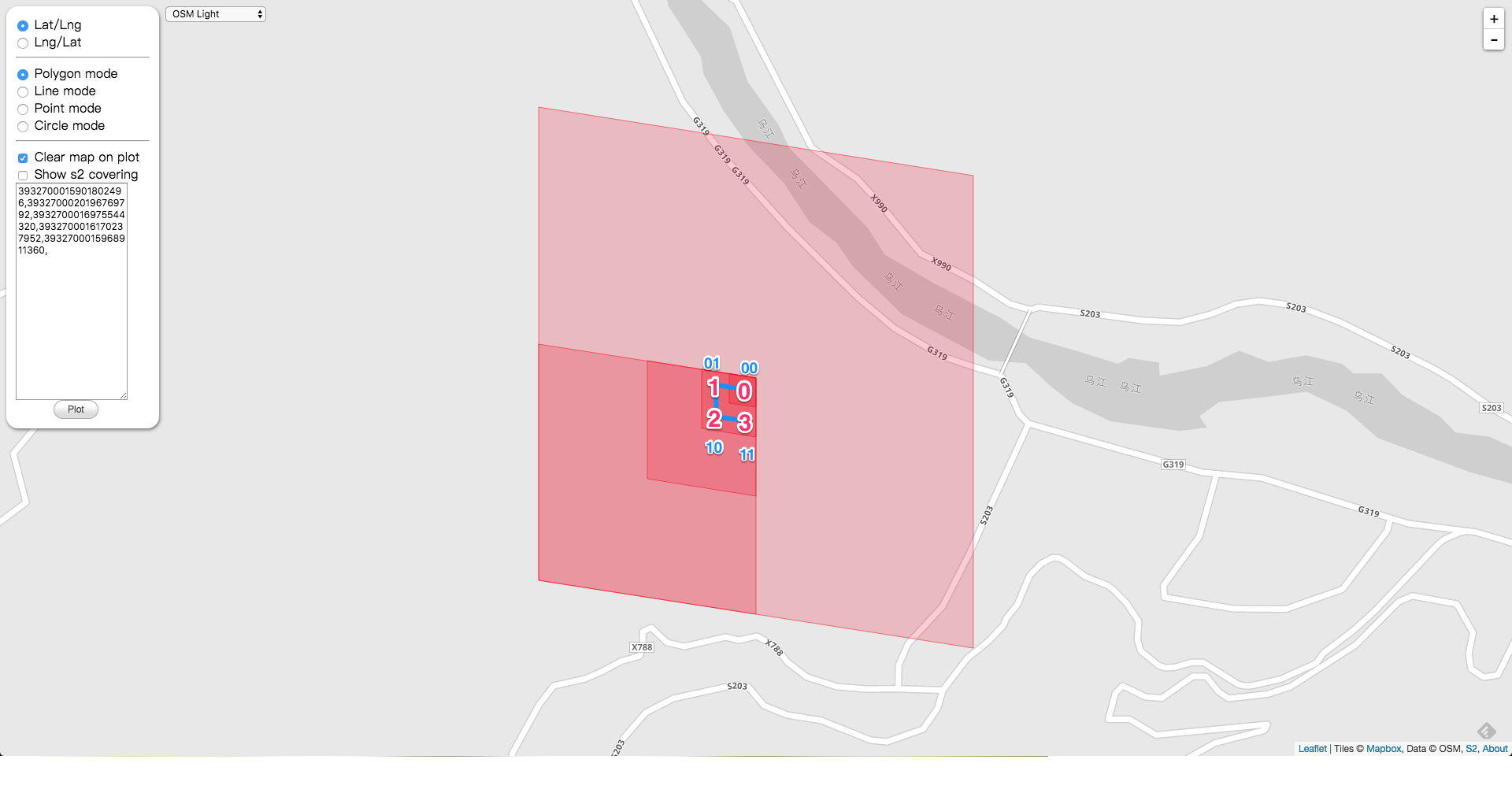
In Figure 0, continue selecting position 0. Therefore, for Level 17, fill the 28th and 29th bits from right to left, calculated as 64 - 3 - 1 - 16 * 2 = 28, with 00. This gives us Level 17.
11011010010011110000011101010000010000000000000000000000000000   16
11011010010011110000011101010000000100000000000000000000000000   17
By the same token, the other child nodes can all be derived using this method.
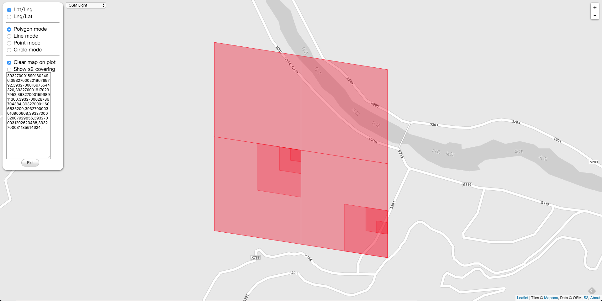
Starting from Level 13, since the orientation corresponding to Level 13 is that of Figure 0 and position 3 is currently selected, we can obtain Level 14. Therefore, the two bits immediately before Level 14’s trailing marker bit 1 are 11. Thus, we can transform from Level 13 to Level 14.
11011010010011110000011101010000000000000000000000000000000000   13 3932700015901802496
11011010010011110000011101011100000000000000000000000000000000   14 3932700028786704384
Since Figure 0 selects position 3, the direction for Level 14 is Figure 3.
The direction corresponding to Level 14 is Figure 3. With position 3 currently selected, Level 15 can be obtained, so the two bits before the trailing flag bit 1 in Level 15 are 11. Thus, Level 14 can be transformed into Level 15.
11011010010011110000011101011100000000000000000000000000000000   14 3932700028786704384
11011010010011110000011101011111000000000000000000000000000000   15 3932700032007929856
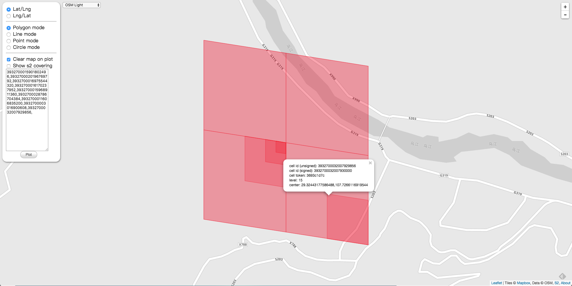
Since position 3 is selected in Figure 3, the direction for Level 15 is Figure 0.
The direction corresponding to Level 15 is Figure 0. Selecting position 0 yields Level 16, so the two bits before the trailing flag bit 1 in Level 16 are 00. Thus, we can transform Level 15 into Level 16.
11011010010011110000011101011111000000000000000000000000000000   15 3932700032007929856
11011010010011110000011101011110010000000000000000000000000000   16 3932700031202623488
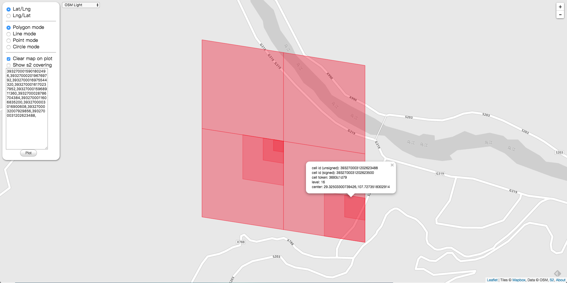
Since Figure 0 selects position 0, the direction for Level 16 is Figure 1.
The direction corresponding to Level 16 is Figure 1. Selecting position 1 at this point yields Level 17, so the two bits before the trailing flag bit 1 in Level 17 are 01. Thus, Level 16 can be transformed into Level 17.
11011010010011110000011101011110010000000000000000000000000000   16 3932700031202623488
11011010010011110000011101011110001100000000000000000000000000   17 3932700031135514624
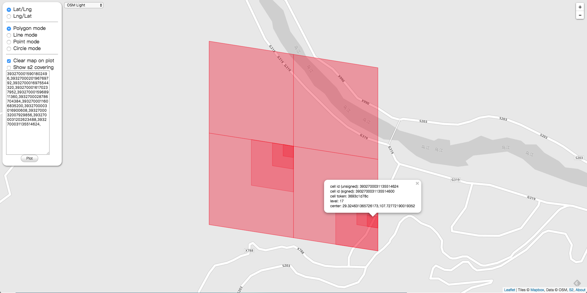
Since Figure 1 selected position 1, the orientation at Level 18 is still Figure 1.
At this point, readers should have a clear understanding of the process for finding the child nodes of a CellID. In Google S2, the concrete implementation for finding child nodes is as follows.
func (ci CellID) Children() [4]CellID {
	var ch [4]CellID
	lsb := CellID(ci.lsb())
	ch[0] = ci - lsb + lsb>>2
	lsb >>= 1
	ch[1] = ch[0] + lsb
	ch[2] = ch[1] + lsb
	ch[3] = ch[2] + lsb
	return ch
}
Now this code should be easy to understand.
The key bitwise operation here is lsb. You can probably tell what it does from the name.
// lsb returns the least significant bit
func (ci CellID) lsb() uint64 { return uint64(ci) & -uint64(ci) }
One thing to note here is that negative numbers are stored as the two’s complement of their sign-magnitude representation: the sign bit remains unchanged, each bit is inverted, and then 1 is added.
For example, a Level 16 CellID is as follows:
11011010010011110000011101011110010000000000000000000000000000 16 3932700031202623488
Compute its LSB:
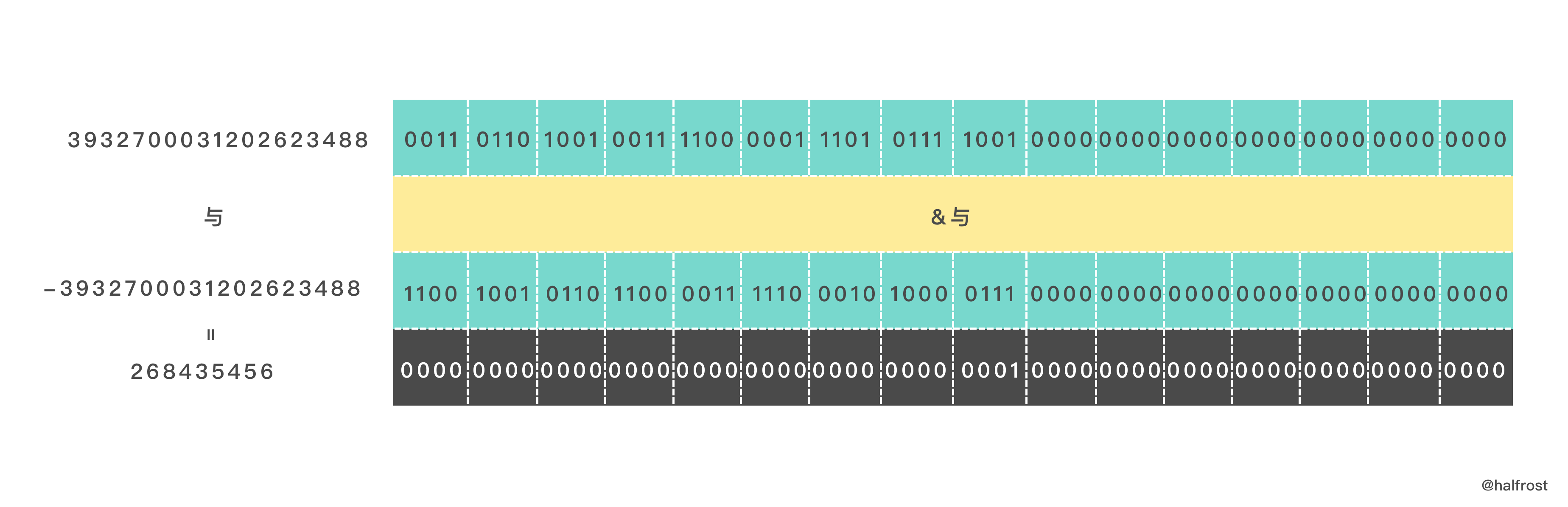
The result is that the least significant bit is 1, and every other bit is 0.
ch[0] = ci - lsb + lsb>>2
This line effectively moves the trailing sentinel bit 1 of the next lower Level corresponding to the current Level into position—that is, shifts it back by 2 bits. Since the two bits before the sentinel bit are both 0, after this operation is completed, the result is the child at index 0.
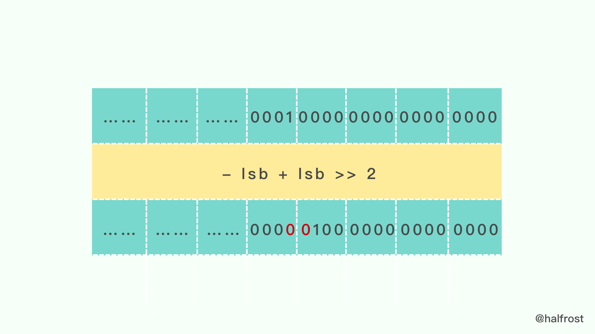
Once child 0 has been found, the rest is straightforward. After shifting lsb one bit to the right, repeatedly adding this value yields the remaining four children, as shown below:
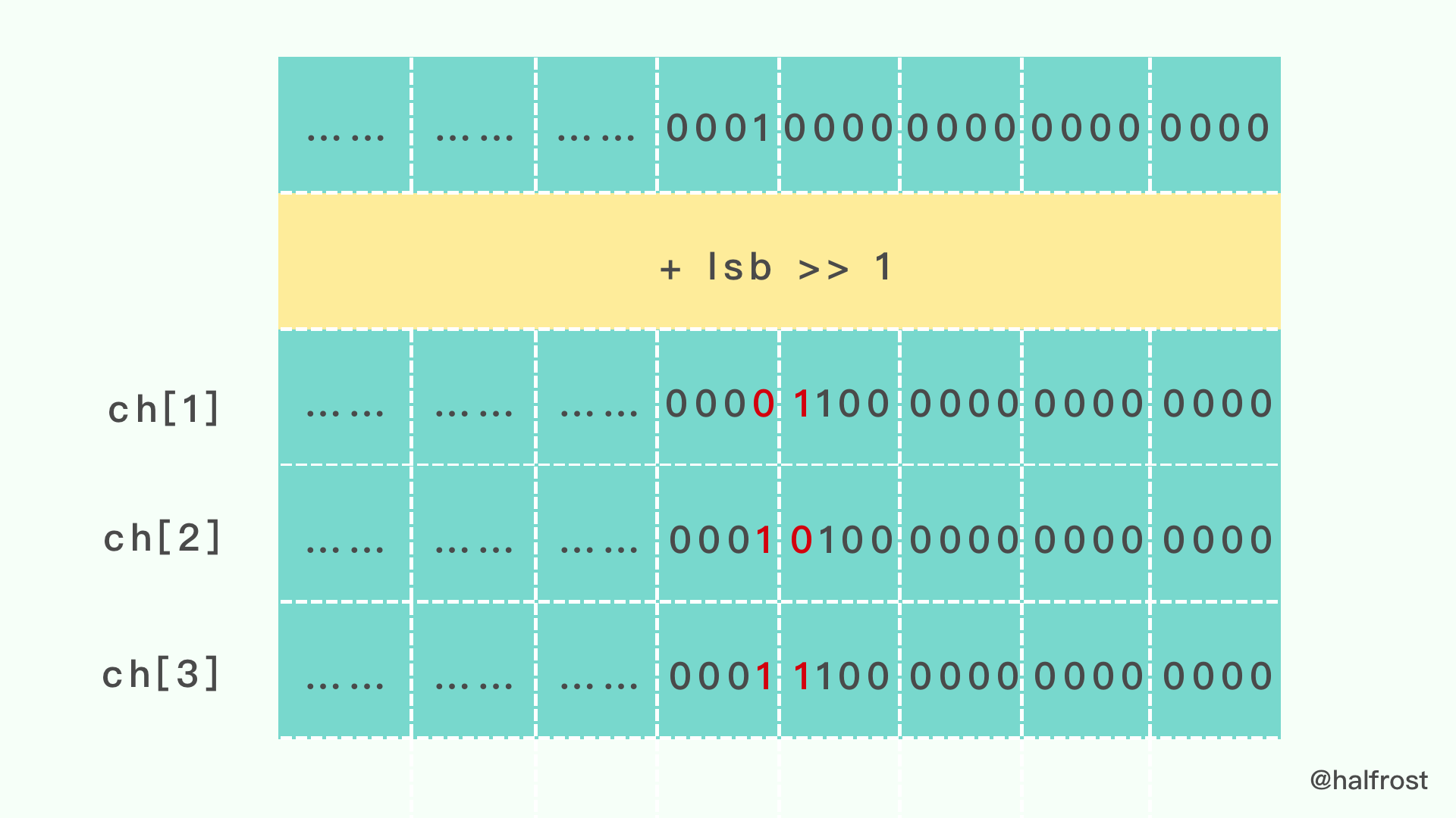
In this way, the four children can be obtained. The short piece of code above is quite simple—even simpler than the earlier explanation based on the map. The reason is that it does not visualize the relative positions of the four children; that relationship must be determined by the current direction. The earlier map repeatedly emphasized the directional relationship at each level in order to visualize on the map the relative positions that conform to the Hilbert curve.
2. Determine Whether It Is a Leaf Node
If you are familiar with the CellID data structure, this check is very simple.
func (ci CellID) IsLeaf() bool { return uint64(ci)&1 != 0 }
Because CellID is 64-bit, it has a trailing 1 marker bit. If this marker bit is in the last position, it must be a leaf node, that is, a Level 30 Cell.
3. Determine the current child’s positional relationship
As described earlier when looking up child nodes, because this is a quadtree, each parent has 4 corresponding children: 00, 01, 10, and 11. Therefore, to determine the relative positional relationship among the 4 children, you only need to check these two binary bits.
func (ci CellID) ChildPosition(level int) int {
	return int(uint64(ci)>>uint64(2*(maxLevel-level)+1)) & 3
}
The input parameter of the function above is the Level of a parent node, and it returns the positional information of a child node under that parent. That is, one of 00, 01, 10, or 11.
4. Finding the Parent Node
In Google S2, because the generated Cell defaults to Level 30, which is the lowest Level, it is a leaf node at the bottom of the tree. Therefore, to generate a Cell with a lower Level, you can only look up its parent node.
As explained earlier, finding a child node works one way; finding the parent node is the reverse process.
func lsbForLevel(level int) uint64 { return 1 << uint64(2*(maxLevel-level)) }
The first step is to find the rightmost flag bit, which determines the value of Level.
(uint64(ci) & -lsb)
The second step is to preserve the values of all binary bits before the flag bit. This can be done by performing a bitwise AND with the negation of lsb from the first step. The negation of lsb is effectively a mask where all higher bits to the left of the low bit of lsb are 1.
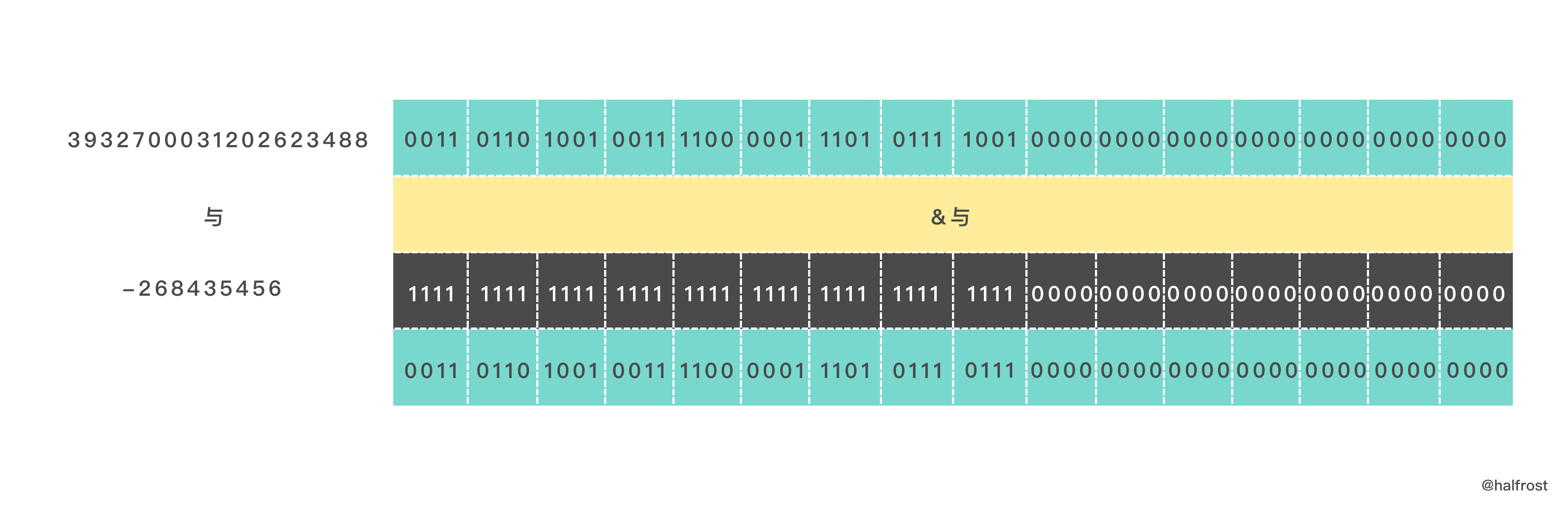
The final step is simply to place the flag bit 1 in the correct position.
func (ci CellID) Parent(level int) CellID {
	lsb := lsbForLevel(level)
	return CellID((uint64(ci) & -lsb) | lsb)
}
That concludes the concrete implementation for finding the parent node.
2. LCA: Finding the Lowest Common Ancestor
For computing a CellID, another critical part is finding the lowest common ancestor. Problem context: given the CellIDs of any two levels in a quadtree, how do we find their lowest common ancestor?
From the data structure of CellID, we know that finding the lowest common ancestor of two levels can be transformed into finding the longest common prefix of two binary strings from left to right. The longest common prefix corresponds to the farthest common ancestor from the root node, which is also the lowest common ancestor.
So the problem now becomes finding the first differing bit from left to right, or equivalently, finding the last differing bit from right to left.
There is a special case in this lookup process: the two nodes whose common ancestor we want to find may already lie on the same branch. That is, one CellID may already be an ancestor of the other CellID. In that case, their common ancestor is simply the larger CellID.
At this point, we can determine the lookup procedure that follows.
First, XOR the two CellIDs to identify the positions of the differing bits.
bits := uint64(ci ^ other)
Second, check for the special case: the two are in an ancestor-descendant relationship.
	if bits < ci.lsb() {
		bits = ci.lsb()
	}
	if bits < other.lsb() {
		bits = other.lsb()
	}
Step 3: find the position of the most significant differing bit.
func findMSBSetNonZero64(bits uint64) int {
	val := []uint64{0x2, 0xC, 0xF0, 0xFF00, 0xFFFF0000, 0xFFFFFFFF00000000}
	shift := []uint64{1, 2, 4, 8, 16, 32}
	var msbPos uint64
	for i := 5; i >= 0; i-- {
		if bits&val[i] != 0 {
			bits >>= shift[i]
			msbPos |= shift[i]
		}
	}
	return int(msbPos)
}
Because CellID is 64 bits, the possible range for the number of differing bits is [0, 63]. Prepare six masks, corresponding to 0x2, 0xC, 0xF0, 0xFF00, 0xFFFF0000, and 0xFFFFFFFF00000000, respectively, as shown below.
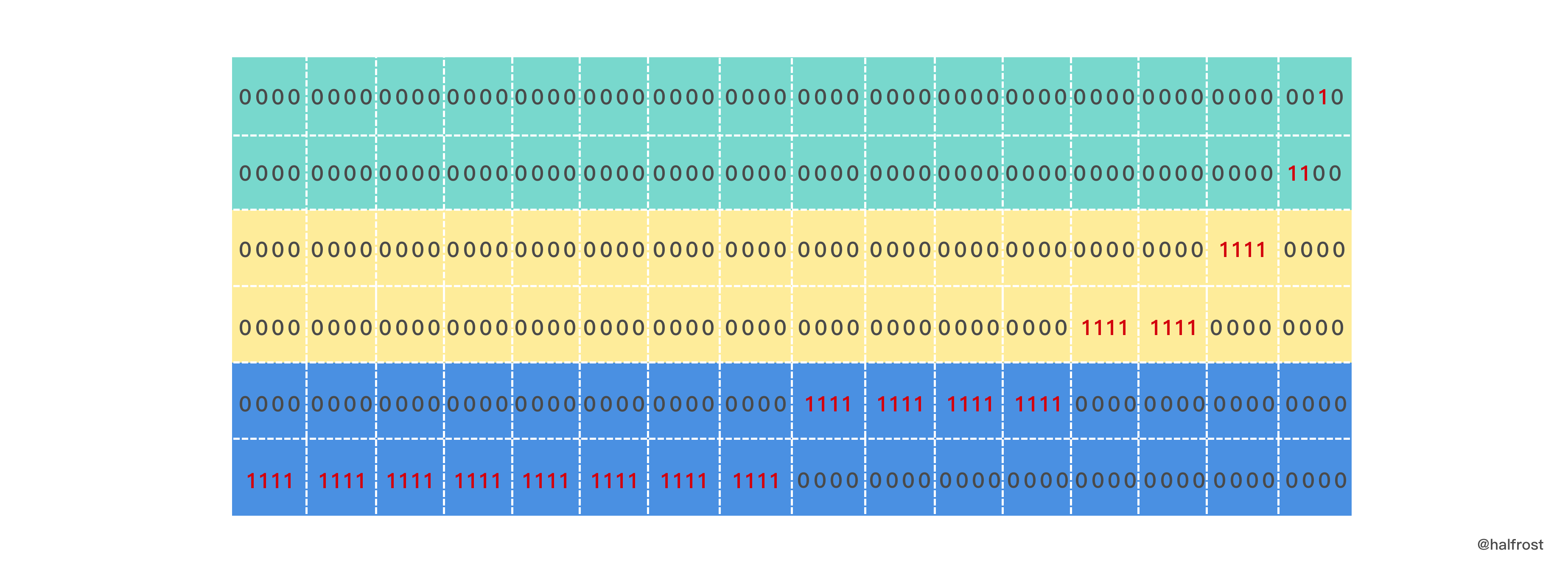
The lookup process uses the idea of binary search. For the 64-bit value, first check the upper 32 bits. If the result of applying the mask to the upper 32 bits with a bitwise AND is non-zero, it means that there are differing bits in the upper 32 bits. In that case, add 32 to the final result msbPos, and shift the number right by 32 bits. Since the upper 32 bits contain differing bits, and what we need is the leftmost one, the lower 32 bits can be discarded directly by shifting right.
Similarly, continue bisecting: 16 bits, 8 bits, 4 bits, 2 bits, and 1 bit. After this loop completes, the leftmost differing bit is guaranteed to be found, and the resulting bit position is msbPos.
The fourth step is to validate msbPos and output the final result.
If msbPos is greater than 60, it is an invalid value, so simply return false.
	msbPos := findMSBSetNonZero64(bits)
	if msbPos > 60 {
		return 0, false
	}
	return (60 - msbPos) >> 1, true
The final output is the Level value of the lowest common ancestor, so after 60 - msbPos, it still needs to be divided by 2.
The complete algorithm implementation is as follows:
func (ci CellID) CommonAncestorLevel(other CellID) (level int, ok bool) {
	bits := uint64(ci ^ other)
	if bits < ci.lsb() {
		bits = ci.lsb()
	}
	if bits < other.lsb() {
		bits = other.lsb()
	}

	msbPos := findMSBSetNonZero64(bits)
	if msbPos > 60 {
		return 0, false
	}
	return (60 - msbPos) >> 1, true
}
For example:
In the example above, we select CellIDs from two Levels that do not have an ancestor relationship.
11011010010011110000011101010000000100000000000000000000000000   17
11011010010011110000011101011111000000000000000000000000000000   15
If we look for the lowest common ancestor directly in this binary string, we can see that the longest common binary string from left to right is:
1101101001001111000001110101
Then their lowest common ancestor is:
11011010010011110000011101010000000000000000000000000000000000
The corresponding Level is 13, and the CellID is 3932700015901802496.
Spatial Search Series:
Understanding n-Dimensional Space and n-Dimensional Spacetime
Efficient Multidimensional Spatial Point Indexing Algorithms — Geohash and Google S2
Finding the LCA (Lowest Common Ancestor) in the Quadtree of Google S2
GitHub Repo: Halfrost-Field
Follow: halfrost · GitHub