How Does Google S2 Solve the Optimal Spatial Coverage Problem?
Preface
Barring any surprises, this will be the final article in the entire Google S2 series. In this article, I’ll explain the regionCoverer algorithm in full. As for the many other small algorithms in the Google S2 library, their code is likewise well worth reading and learning from, but I won’t go through them one by one here. Interested readers can read through the entire library.
While writing this article, I noticed some new commits from the library’s author, such as commit f9610db2b871b54b17d36d4da6a4d6a2aab6018d from December 4, 2017. That commit changed the README; although it looks like it only modifies documentation, there is actually a lot of substance in it.
 -For an analogous library in C++, see
 -https://code.google.com/archive/p/s2-geometry-library/, and in Java, see
 -https://github.com/google/s2-geometry-library-java
------------------------------------------------------------------------------------
 +For an analogous library in C++, see https://github.com/google/s2geometry, in
 +Java, see https://github.com/google/s2-geometry-library-java, and Python, see
 +https://github.com/google/s2geometry/tree/master/src/python
You can see that they moved the code that used to live in Google’s official private code repository to GitHub. Previously, the C++ code could only be viewed in the code archives; now it can be viewed directly on GitHub, which is much more convenient.
+More details about S2 in general are available on the S2 Geometry Website
 +[s2geometry.io](https://s2geometry.io/).
This commit also mentions a new website, which I found was only recently launched. I have been following every S2 commit continuously for nearly half a year, and I keep an eye on every S2-related resource online, so this site is very new. I’ll mention this website at the end of the article, so I won’t go into detail here.
Starting with this commit, I believe Google S2 may be getting more attention, and it is also possible that there are plans to promote it more aggressively.
All right, let’s get to the main topic.
I. Spatial Types
In Google S2, the following types can be used for RegionCovering. Basically, they all need to satisfy the Region interface.
1. Cap
Cap represents a disk-shaped region defined by a center and a radius. Technically, this shape is called a “spherical cap” rather than a disk, because it is not planar. A cap represents the portion of a sphere cut off by a plane. The boundary of a cap is the circle defined by the intersection of the sphere and the plane. A cap is a closed set, meaning it includes its boundary. In most cases, wherever you would use a disk in planar geometry, you can use a spherical cap. The radius of a cap is measured along the surface of the sphere, rather than as a straight-line distance through the interior. Therefore, a cap with radius π/2 is a hemisphere, and a cap with radius π covers the entire sphere. The center is a point on the unit sphere. (Therefore, it must have unit length.) A cap can also be defined by its center point and height. The height is the distance from the center point to the cutting plane. There is also support for “empty” and “full” caps, containing no points and all points respectively. Below are some useful relationships among cap height (h), cap radius (r), maximum chord length from the cap center (d), and the radius of the cap base (a).
h = 1 - cos(r)
	= 2 * sin^2(r/2)
d^2 = 2 * h
	= a^2 + h^2
2. Loop
A Loop represents a simple spherical polygon. It consists of a sequence of vertices, where the first vertex is implicitly considered to be connected to the last vertex. All loops are defined to have CCW orientation; that is, the interior of the loop is on the left side of its edges. This means that a clockwise loop enclosing a small area is interpreted as a CCW loop enclosing a very large area. A loop may not have any duplicate vertices, whether adjacent or not. Adjacent edges may not intersect, and edges of length 180 degrees are not allowed (that is, adjacent vertices cannot be antipodal). A loop must have at least 3 vertices, except for the “empty” and “full” loops discussed below. There are two special loops: EmptyLoop contains no points, and FullLoop contains all points. These loops do not have any edges, but in order to preserve the invariant that every loop can be represented as a vertex chain, they are defined to have one vertex each.
3. Polygon
A Polygon represents a sequence of zero or more loops; similarly, the left-hand side of a loop’s direction is defined as its interior. When a polygon is initialized, the given loops are automatically converted into a canonical form consisting of “holes”. The loops are reordered to correspond to a predefined traversal of the nesting hierarchy. A polygon can represent any region of the sphere with a polygonal boundary, including the entire sphere (called a “full” polygon). A full polygon consists of one full loop, while an empty polygon has no loops at all. Use FullPolygon() to construct a full polygon. The zero value of Polygon is treated as an empty polygon.
For multiple loops to form a Polygon, the following 4 conditions must be satisfied:
- Loops must not cross; that is, the boundary of a loop may not intersect both the interior and exterior of any other loop.
- Loops must not share edges; that is, if a loop contains edge AB, no other loop may contain AB or BA.
- Loops may share vertices, but no vertex may appear twice within a single loop (see S2Loop).
- Empty loops are not allowed. A full loop may appear only in a full polygon.
4. Rect
Rect represents a closed latitude-longitude rectangle. It is also a Region type. It can represent empty and full rectangles as well as a single point. It has an AddPoint method, which makes it convenient to construct a bounding rectangle for a set of points, including point sets that span the 180-degree meridian.
5. Region
A Region represents a two-dimensional region on the unit sphere. The purpose of this interface is to approximate complex regions with simpler ones. The interface is limited to methods for computing approximations.
An S2 Region represents a two-dimensional region on the unit sphere. It is an abstract interface with various concrete subtypes, such as disks, rectangles, polylines, polygons, geometry collections, buffered shapes, and so on. The primary purpose of this interface is to allow complex regions to be approximated by simpler regions. Therefore, the interface should only be used for methods that compute approximations, rather than as a broad set of virtual methods implemented by all subtypes.
6. Shape
Shape can be regarded as the “base class” for all geometries or shapes. It represents geometric polygons in the most flexible way. It is composed of a set of edges and optionally defines an interior. All geometries represented by a given Shape must have the same dimension, which means a Shape can represent a set of points, a set of polylines, or a set of polygons. Shape is defined as an interface so that clients can more conveniently control the underlying data representation. Sometimes a Shape does not own its data, but instead wraps data of other types. Shape operations are usually defined on ShapeIndex rather than on individual shapes. A ShapeIndex is simply a collection of Shapes, possibly with different dimensions (for example, 10 points and 3 polygons), organized into a data structure for efficient access. The edges of a Shape are indexed by edge IDs in a contiguous range starting from 0. Edges are further subdivided into chains, where each chain consists of a sequence of edges connected end-to-end (a polyline). For example, a shape representing two polylines AB and CDE would have three edges (AB, CD, DE) divided into two chains (AB) and (CD, DE). Similarly, a shape representing 5 points would have 5 chains, each consisting of one edge. Shape has methods that allow edges to be accessed using either a global number (edge ID) or within a specific chain. Global numbering is sufficient for most cases, but the chain representation is very useful for certain algorithms, such as intersection (see BooleanOperation).
S2 defines two extensible interfaces for representing geometry in total: S2Shape and S2Region.
The difference between them is: The purpose of S2Shape is to flexibly represent polygonal geometry. (This includes not only polygons, but also points and polylines.) Most core S2 operations work with any class that implements the S2Shape interface.
The purpose of S2Region is to compute approximations of geometry. For example, there are methods for computing bounding rectangles and disks, and S2RegionCoverer can be used to approximate a region, to any desired precision, as a collection of cells. Unlike S2Shape, S2Region can represent non-polygonal geometries, such as spherical caps (S2Cap).
In addition to the commonly used types described above, the following intermediate or lower-level types are also available for developers to use.
- S2LatLngRect - A rectangle in the latitude-longitude coordinate system.
- S2Polyline - A polyline.
- S2CellUnion - A region approximated as a collection of S2CellIds. This is the type produced after conversion by RegionCoverer.
- S2ShapeIndexRegion - An arbitrary collection of points, polylines, and polygons.
- S2ShapeIndexBufferedRegion - Defined the same way as S2ShapeIndexRegion, except expanded by a given radius.
- S2RegionUnion - A collection of arbitrary regions.
- S2RegionIntersection - The intersection of arbitrary other regions.
Finally, as an additional note, the S2RegionTermIndexer type supports indexing and querying any type of S2Region, namely all the types mentioned above. You can use S2RegionTermIndexer to index a set of polylines and then query which polylines intersect a given polygon.
II. RegionCoverer Examples
RegionCoverer is mainly intended to find an approximately optimal solution that can cover the current region (why not an optimal solution?).
There are mainly 3 conversion parameters: MaxLevel, MaxCells, and MinLevel. MaxCells determines the maximum number of cells, but getting too close to the maximum can cause the covered area to become too large and imprecise. Therefore, the maximum count is only a limit on the maximum number allowed while satisfying the maximum precision. Because of this, the result is not necessarily the optimal solution satisfying MaxCells.
A few examples:
The following is a cap with a radius of 10 kilometers, and this cap is located at the corner where 3 faces meet. Suppose we need at most 10 cells to cover it. The result is as follows:
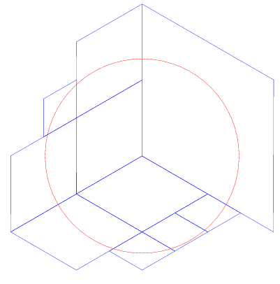
With the same settings, we change the count to 20, as follows:
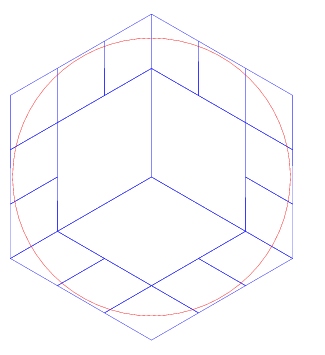
Still using the same configuration, change the count to 50:
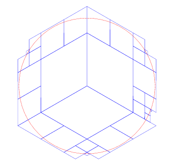
So far, the accuracy is just so-so; the edges still cover more than the original cap. We continue improving the precision by adjusting the count to 200.
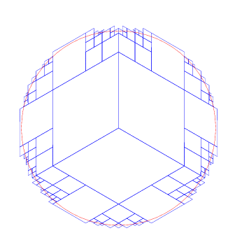
200 cells appears relatively precise. Let’s increase it again to 1000 and see what happens.
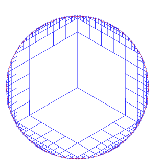
Although the code configuration sets 1000 cells, there are actually only 706 cells. The reason is that although the code computes based on 1000 cells, the actual algorithm also merges cells after pruning. Therefore, the final count is less than 1000.
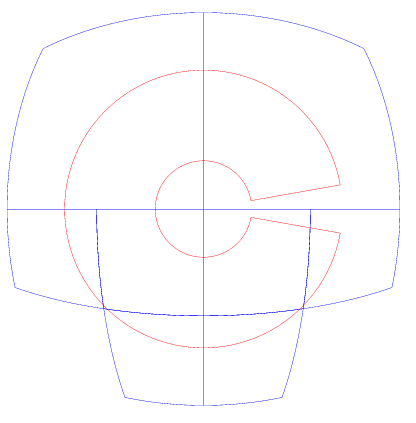
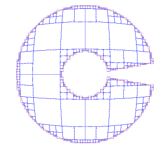
Let’s look at another example. The rectangle below represents a latitude/longitude rectangle extending from 60 degrees north latitude to 80 degrees north latitude, and from -170 degrees longitude to +170 degrees. The covering is limited to 8 cells. Note that the hole in the middle is completely covered. This is clearly not what we intended.
We increase the number of cells to 20. The hole in the middle is still filled in.
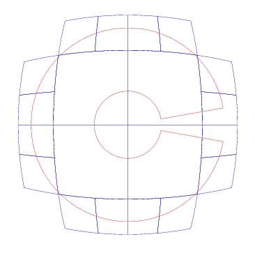
We adjust the parameter to 100 while keeping all other configuration exactly the same. Now the hole in the middle has begun to take shape. However, the gap near the date line still does not appear.
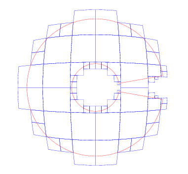
Finally, we adjust the parameter to 500. Now the hole in the middle is displayed relatively completely.
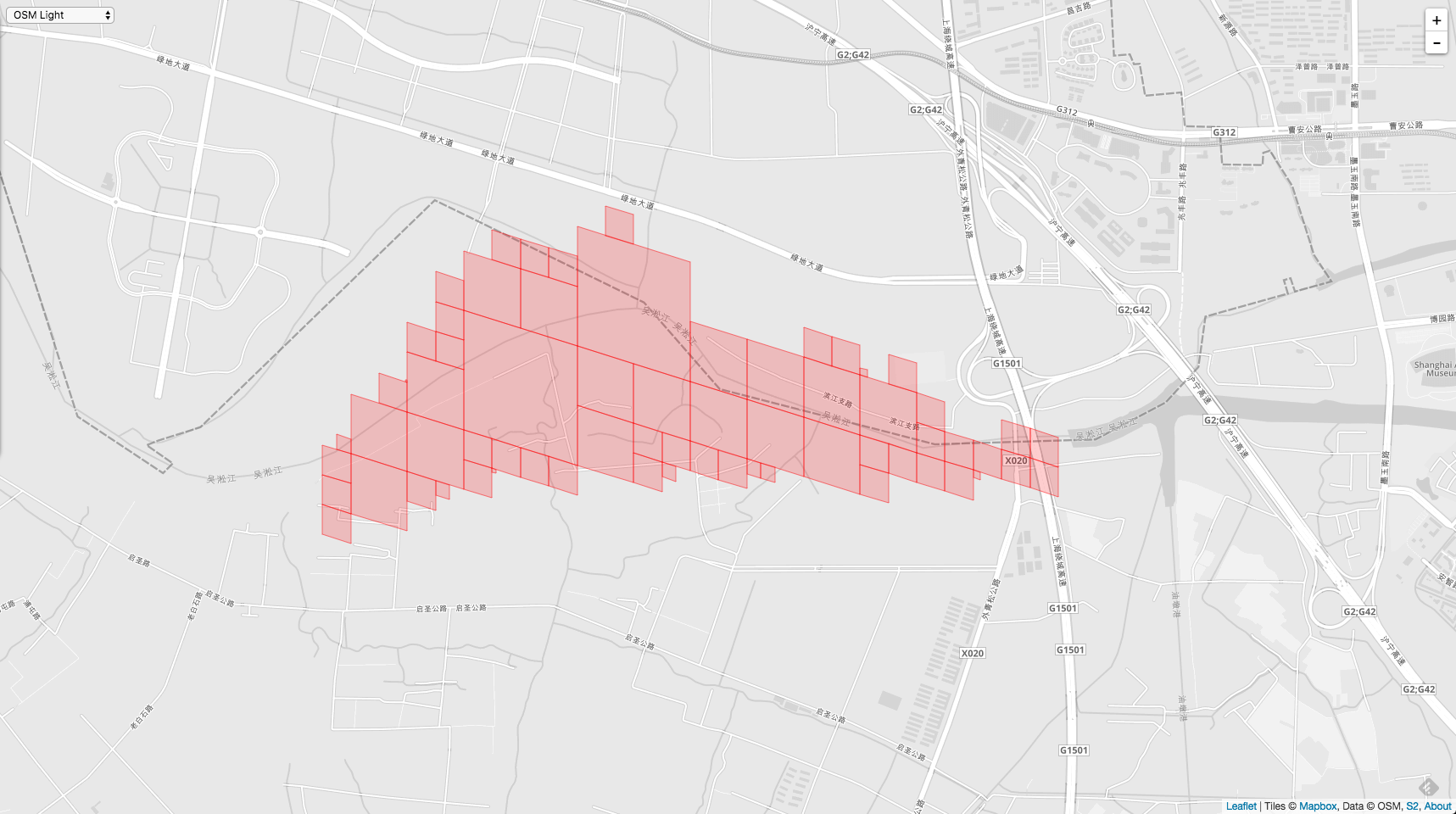
Here are a few more examples from our actual project. The following is the edge of a grid in Shanghai. First, we use
defaultCoverer := &s2.RegionCoverer{MaxLevel: 16, MaxCells: 100, MinLevel: 13}
After conversion, the result is as follows:
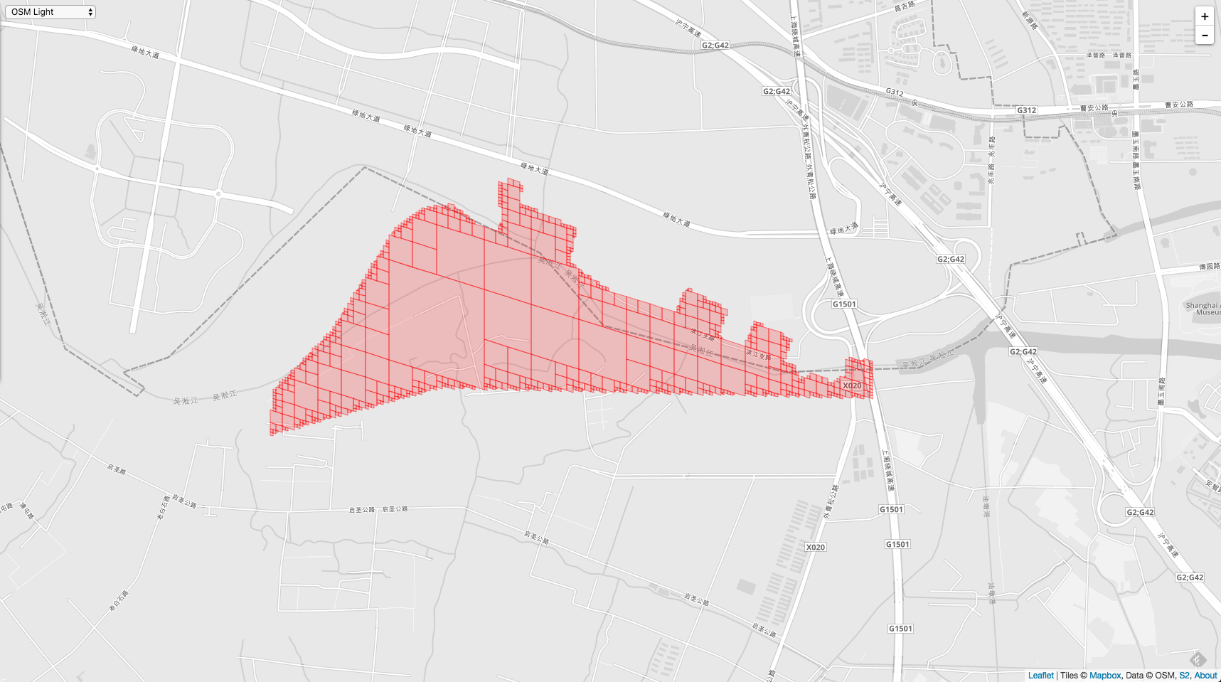
defaultCoverer := &s2.RegionCoverer{MaxLevel: 30, MaxCells: 1000, MinLevel: 1}
When the precision is increased to 1000, the result looks like this:
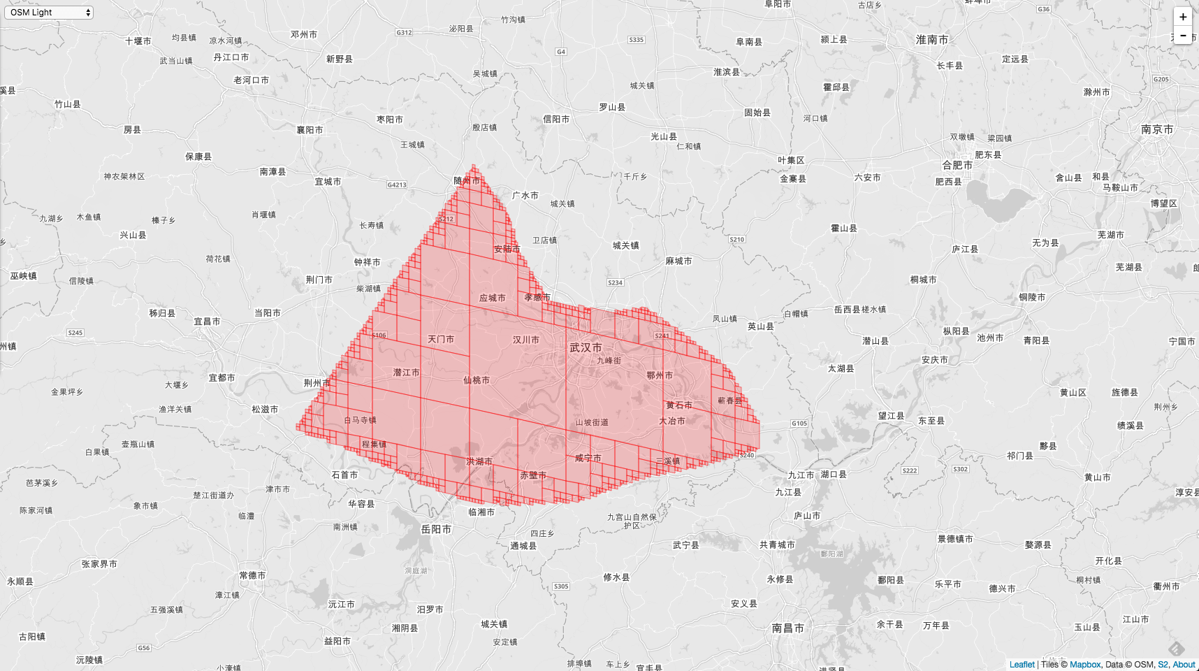
There are also cases with larger regions, such as a province—Hubei Province:
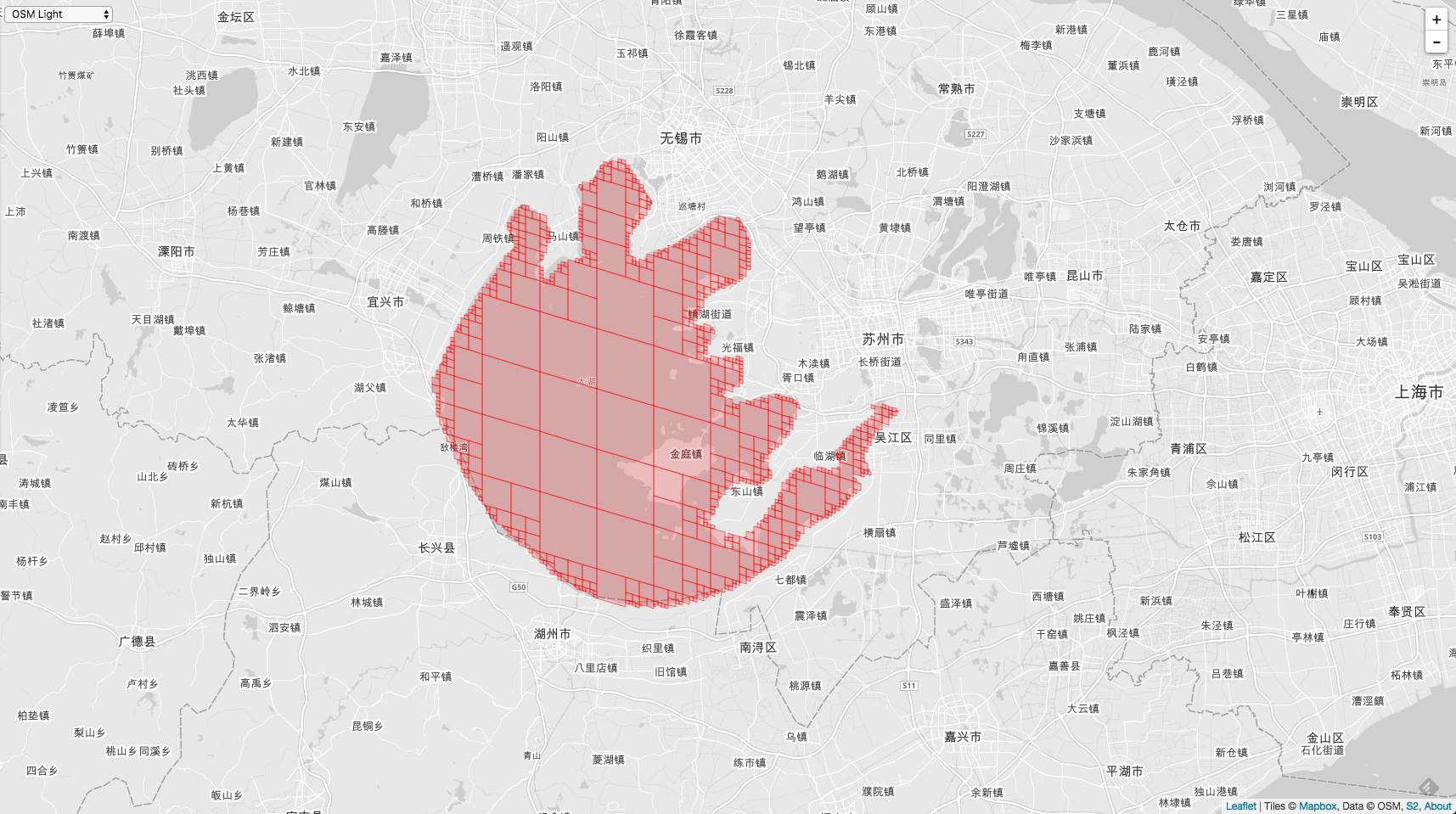
Or a lake—Taihu Lake:
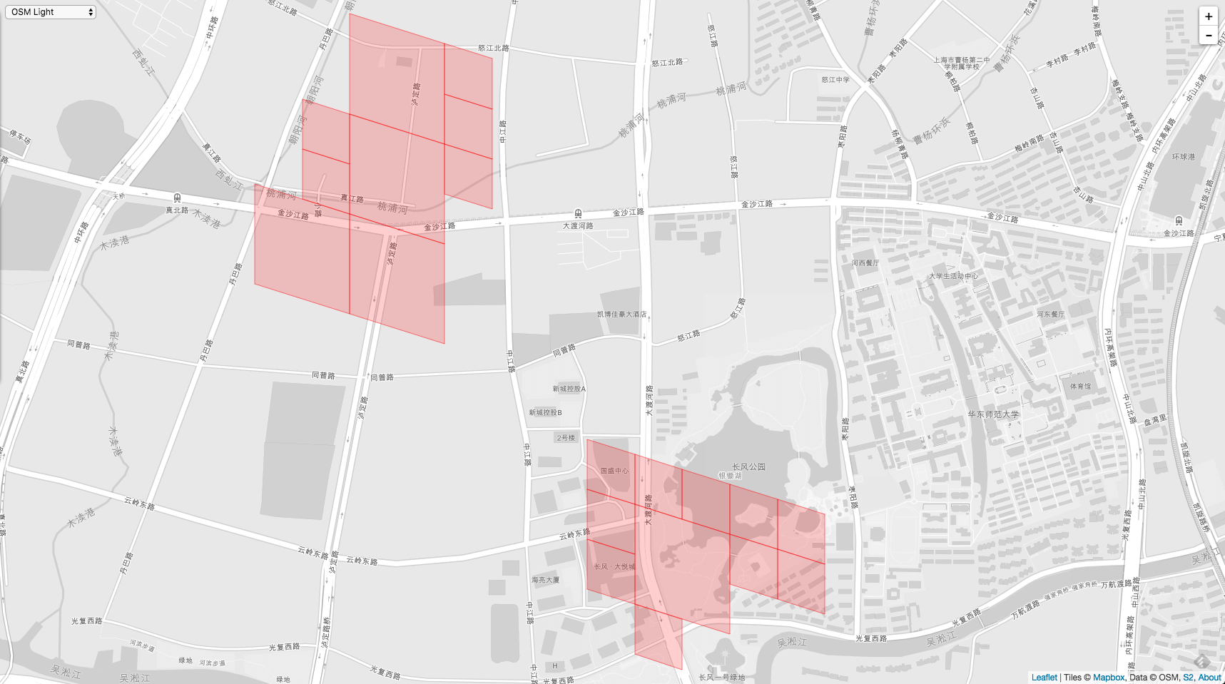
Finally, here is another polygon example. We know that a polygon consists of multiple loops:
	loops := []*s2.Loop{}
	loops = append(loops, loop1)
	loops = append(loops, loop2)

	polygon := s2.PolygonFromLoops(loops)

	defaultCoverer := &s2.RegionCoverer{MaxLevel: 16, MaxCells: 100, MinLevel: 8}
	fmt.Println("----  polygon-----")

	cvr = defaultCoverer.Covering(polygon)

	for i := 0; i < len(cvr); i++ {
		fmt.Printf("%d,\n", cvr[i])
	}
	fmt.Printf("------------\n")
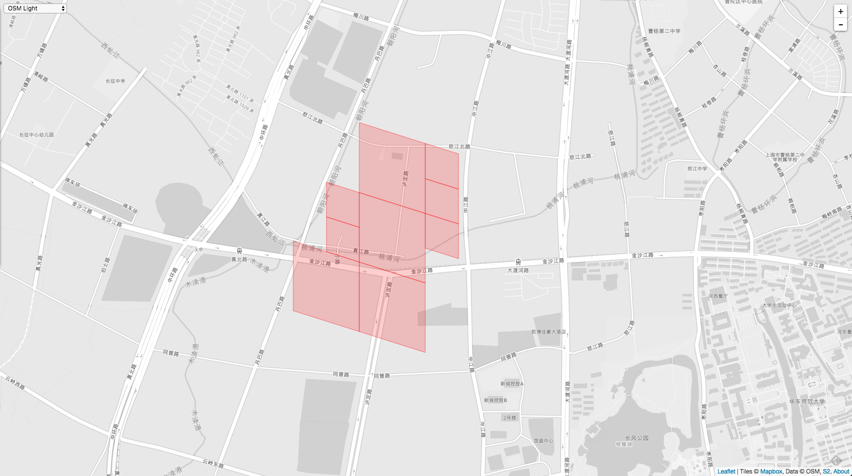
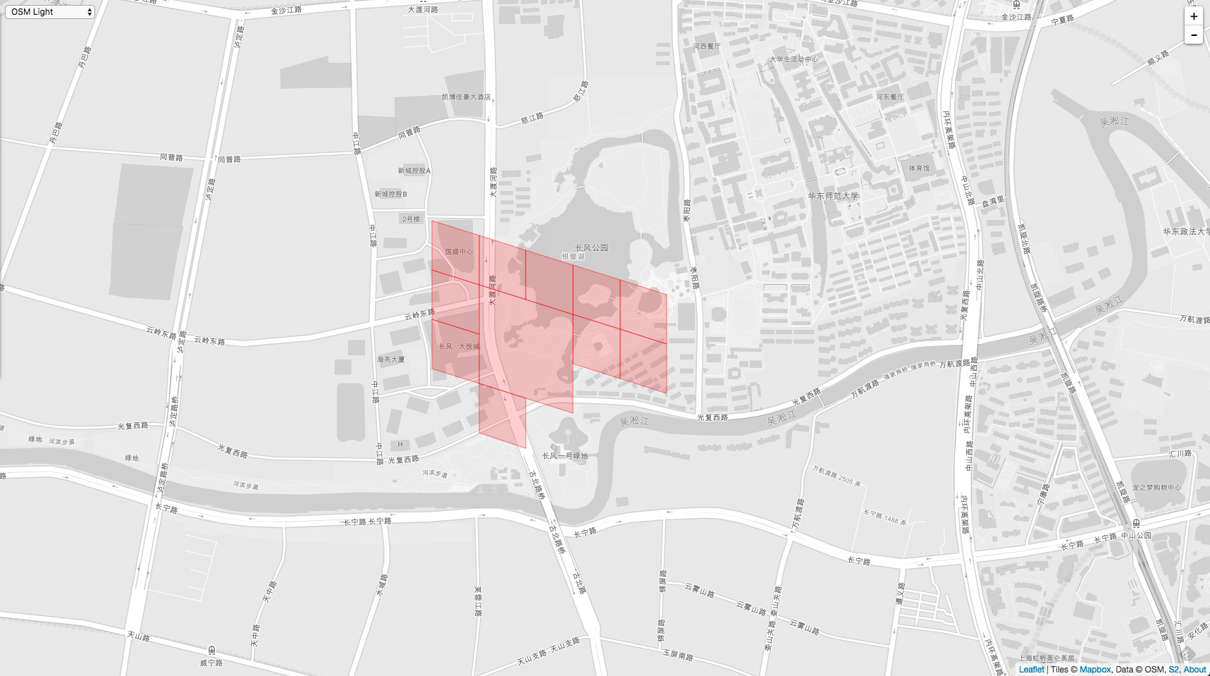
Below are the two loops on the map, respectively.
Finally, here is the polygon, which contains the two loops above.
III. Implementation of the Core RegionCoverer Algorithm: Covering
This section provides a detailed analysis of how Covering is implemented.
The most common usage is just the following few lines:
	rc := &s2.RegionCoverer{MaxLevel: 30, MaxCells: 5}
	r := s2.Region(CapFromCenterArea(center, area))
	covering := rc.Covering(r)
The example above shows that after the maximum conversion, the CellUnion contains 5 CellIDs. The region covered by the three lines above is a Cap.
type RegionCoverer struct {
	MinLevel int // the minimum cell level to be used.
	MaxLevel int // the maximum cell level to be used.
	LevelMod int // the LevelMod to be used.
	MaxCells int // the maximum desired number of cells in the approximation.
}
RegionCoverer is a struct that actually contains four fields: MinLevel, MaxLevel, MaxCells, and LevelMod. The first three should be self-explanatory; they are used frequently. The key point to explain is LevelMod.
Once LevelMod is set, during RegionCover conversion, the selected Cell Level can only satisfy (level - MinLevel) % LevelMod = 0; that is, (level - MinLevel) must be a multiple of LevelMod. Only Cell Levels that meet this condition will be selected. This effectively allows the branching factor of the S2 CellID hierarchy to increase. The current valid parameter values can only be 0, 1, 2, and 3, with corresponding branching factors of 0, 4, 16, and 64.
Now let’s talk about the core idea of the algorithm.
RegionCover can be abstracted as the following problem: given a region, cover it with Cells as accurately as possible, but with the total number not exceeding MaxCells. How do we find those Cells?
This is a greedy, locally optimal problem. If you want maximum precision, the obvious approach is to cover all boundary areas with MaxLevel cells (the larger the Level, the smaller the cells). That gives the highest precision. But it also causes the number of Cells to explode, far exceeding MaxCells, which violates the requirement. So how can we cover the given region as accurately as possible while keeping the count <= MaxCells?
A few points need to be clarified up front:
- MinLevel has higher priority than MaxCells (note: not MaxLevel). In other words, Cells below the given Level will never be used, even if using one of them could replace many smaller-area Cells with larger Levels.
- Regarding the minimum valid range of MaxCells: if a certain case requires a minimum number of units—for example, if the region intersects all six face cells—then up to 6 cells may be returned. If it happens to lie at the intersection of three cube faces, then up to 3 cells may be returned even for a very small cap region.
- If MinLevel is too large even for the approximated region, then MaxCells loses its constraining effect, and any number of cells may be returned.
- If MaxCells is less than 4, then even if the region is convex, such as a cap or rect, the final covered area will be larger than the original region. Developers should be aware of this case.
All right, next let’s start from the source code. The core function for RegionCoverer conversion is this one.
func (rc *RegionCoverer) Covering(region Region) CellUnion {
	covering := rc.CellUnion(region)
	covering.Denormalize(maxInt(0, minInt(maxLevel, rc.MinLevel)), maxInt(1, minInt(3, rc.LevelMod)))
	return covering
}
From this function’s implementation, we can see that the conversion is effectively split into two steps: Normalize Cell + conversion, and Denormalize Cell.
(1). CellUnion
The concrete implementation of the CellUnion method:
func (rc *RegionCoverer) CellUnion(region Region) CellUnion {
	c := rc.newCoverer()
	c.coveringInternal(region)
	cu := c.result
	cu.Normalize()
	return cu
}
This method can also be broken down into three main parts: creating newCoverer, coveringInternal, and Normalize.
1. newCoverer()
func (rc *RegionCoverer) newCoverer() *coverer {
	return &coverer{
		minLevel: maxInt(0, minInt(maxLevel, rc.MinLevel)),
		maxLevel: maxInt(0, minInt(maxLevel, rc.MaxLevel)),
		levelMod: maxInt(1, minInt(3, rc.LevelMod)),
		maxCells: rc.MaxCells,
	}
}
The newCoverer() method initializes a coverer struct. maxLevel is a previously defined constant, with maxLevel = 30. All initialization parameters for coverer come from the parameters of RegionCoverer. We initialize a RegionCoverer externally, and its four main parameters—MinLevel, MaxLevel, LevelMod, and MaxCells—are all passed in here. In the initialization function above, maxInt and minInt are mainly used to handle invalid values.
In fact, the coverer struct contains 8 fields.
type coverer struct {
	minLevel         int // the minimum cell level to be used.
	maxLevel         int // the maximum cell level to be used.
	levelMod         int // the LevelMod to be used.
	maxCells         int // the maximum desired number of cells in the approximation.
	region           Region
	result           CellUnion
	pq               priorityQueue
	interiorCovering bool
}
Excluding the four items initialized above, it actually also includes four other important items, which will be used later. region is the area to be covered. result is the final conversion result, an array of CellUnion. pq is the priority queue priorityQueue, and interiorCovering is a bool variable indicating whether the current conversion is an interior conversion.
2. coveringInternal()
Next, let’s look at the coveringInternal method.
func (c *coverer) coveringInternal(region Region) {
	c.region = region

	c.initialCandidates()
	for c.pq.Len() > 0 && (!c.interiorCovering || len(c.result) < c.maxCells) {
		cand := heap.Pop(&c.pq).(*candidate)

		if c.interiorCovering || int(cand.cell.level) < c.minLevel || cand.numChildren == 1 || len(c.result)+c.pq.Len()+cand.numChildren <= c.maxCells {
			for _, child := range cand.children {
				if !c.interiorCovering || len(c.result) < c.maxCells {
					c.addCandidate(child)
				}
			}
		} else {
			cand.terminal = true
			c.addCandidate(cand)
		}
	}
	c.pq.Reset()
	c.region = nil
}
The coveringInternal method generates the covering plan and stores the result in result. The general strategy for the covering transformation is:
Start with the 6 faces of the cube. Discard any shapes that do not intersect the region. Then repeatedly select the largest cell that intersects the shape and subdivide it.
The coverer struct has 8 fields. The first 4 are initialized from the outside, and the last 4 are used here. First,
c.region = region
Initialize the coverer’s region. The other three elements—result, pq, and interiorCovering—will all be used below.
result only contains qualifying Cells that will become part of the final output, while the pq priority queue contains Cells that may still need to be subdivided further.
If a Cell is 100% fully contained within the covering region, it is immediately added to the output; a Cell that has no intersection with the region at all is immediately discarded. Therefore, the pq priority queue only contains Cells that partially intersect the region.
The dequeue strategy for the pq priority queue is:
1. First, prioritize candidates by Cell size (larger Cells come first)
2. Then by the number of intersecting children (fewer children have higher priority and are dequeued first)
3. Finally, by the number of fully contained children (fewer children have higher priority and are dequeued first)
After filtering through the pq priority queue, the Cells that ultimately remain must have the lowest priority: that is, their Cell area is relatively small, and they have a large overlap with the region and the largest number of fully contained children. In other words, the Cells that lie closest to the region boundary (the Cells whose covered area has the least excess beyond the region to be covered/converted) are the ones that will ultimately remain.
if c.interiorCovering || int(cand.cell.level) < c.minLevel || cand.numChildren == 1 || len(c.result)+c.pq.Len()+cand.numChildren <= c.maxCells {

}
The intent of this condition in the implementation of coveringInternal is:
For an interior covering, no matter how many children a candidate has, we keep subdividing it. If we reach MaxCells before expanding all of its children, we simply use some of them. For an exterior covering, we cannot do this, because the result must cover the entire region, so all children must be used.
candidate.numChildren == 1
In the situation above, we have already handled the case where there are too many MaxCells results (minLevel is too high). In this case, even if a child candidate is further subdivided, it has little impact on the final result.
3. initialCandidates()
Next, let’s look at how candidates are initialized:
func (c *coverer) initialCandidates() {
	// Optimization: start with a small (usually 4 cell) covering of the region's bounding cap.
	temp := &RegionCoverer{MaxLevel: c.maxLevel, LevelMod: 1, MaxCells: min(4, c.maxCells)}

	cells := temp.FastCovering(c.region)
	c.adjustCellLevels(&cells)
	for _, ci := range cells {
		c.addCandidate(c.newCandidate(CellFromCellID(ci)))
	}
}
This function includes a small optimization: the first-pass covering of the region is converted into four Cells that cover the Caps along the region boundary. The two more important methods in the implementation of initialCandidates are FastCovering and adjustCellLevels.
4. FastCovering()
func (rc *RegionCoverer) FastCovering(region Region) CellUnion {
	c := rc.newCoverer()
	cu := CellUnion(region.CellUnionBound())
	c.normalizeCovering(&cu)
	return cu
}
The FastCovering function returns a CellUnion whose Cells cover the given region. What makes this method different is that it is very fast, and the result is relatively coarse. Of course, the resulting CellUnion still satisfies the MaxCells, MinLevel, MaxLevel, and LevelMod constraints. It just does not try to make full use of a large MaxCells value. In general, it returns only a small number of Cells, so the result is fairly coarse.
Therefore, using FastCovering as the starting point for recursively subdividing Cells is very effective.
Inside this method, region.CellUnionBound() is called. How this behaves depends on how each region type implements this interface.
Taking loop as an example, its implementation of CellUnionBound() is as follows:
func (l *Loop) CellUnionBound() []CellID {
	return l.CapBound().CellUnionBound()
}
The method above is the concrete implementation for quickly computing boundary transitions. It is also the core part of implementing spatial coverage.
CellUnionBound returns an array of CellIDs that covers the region. The Cells are not sorted, may contain redundancy (for example, a cell that contains other cells), and may cover more area than necessary.
For this reason, this method is not suitable for direct use by client code. Clients should generally use the Region.Covering method, which can be used to control the size and accuracy of the covering. In addition, if you want fast coverage and do not care about accuracy, consider calling FastCovering (it returns a cleaned-up version of the covering computed by this method).
The CellUnionBound implementation should try to return a small covering of the covered region (ideally 4 cells or fewer) and be fast to compute. Therefore, the CellUnionBound method is used by RegionCoverer as the starting point for further refinement.
func (l *Loop) CapBound() Cap {
	return l.bound.CapBound()
}
CapBound returns an upper bound on the boundary, which may include more padding than the corresponding RectBound. Its bound is conservative: if the loop contains point P, then the bound is guaranteed to contain that point as well.
func (c Cap) CellUnionBound() []CellID {

	level := MinWidthMetric.MaxLevel(c.Radius().Radians()) - 1

	// If level < 0, more than three face cells are required.
	if level < 0 {
		cellIDs := make([]CellID, 6)
		for face := 0; face < 6; face++ {
			cellIDs[face] = CellIDFromFace(face)
		}
		return cellIDs
	}

	return cellIDFromPoint(c.center).VertexNeighbors(level)
}
The code above is the core algorithm of the roughest version of the conversion. In this algorithm, the key step is computing the level we need to find.
level := MinWidthMetric.MaxLevel(c.Radius().Radians()) - 1
The Level found here is the largest Cell that this Cap can contain.
return cellIDFromPoint(c.center).VertexNeighbors(level)
The line above returns 4 Cells, the ones closest to the center point of the Cap. Of course, if the Cap is very large, it may return 6 Cells. The returned Cells are not sorted in any way.
5. normalizeCovering()
The final step of FastCovering is normalizeCovering.
func (c *coverer) normalizeCovering(covering *CellUnion) {
	// 1
	//
	if c.maxLevel < maxLevel || c.levelMod > 1 {
		for i, ci := range *covering {
			level := ci.Level()
			newLevel := c.adjustLevel(minInt(level, c.maxLevel))
			if newLevel != level {
				(*covering)[i] = ci.Parent(newLevel)
			}
		}
	}
	// 2
	//
	covering.Normalize()

	// 3
	//
	for len(*covering) > c.maxCells {
		bestIndex := -1
		bestLevel := -1
		for i := 0; i+1 < len(*covering); i++ {
			level, ok := (*covering)[i].CommonAncestorLevel((*covering)[i+1])
			if !ok {
				continue
			}
			level = c.adjustLevel(level)
			if level > bestLevel {
				bestLevel = level
				bestIndex = i
			}
		}

		if bestLevel < c.minLevel {
			break
		}
		(*covering)[bestIndex] = (*covering)[bestIndex].Parent(bestLevel)
		covering.Normalize()
	}
	// 4
	//
	if c.minLevel > 0 || c.levelMod > 1 {
		covering.Denormalize(c.minLevel, c.levelMod)
	}
}
normalizeCovering further normalizes the covering transformation result from the previous step so that it conforms to the current covering parameters (MaxCells, minLevel, maxLevel, and levelMod). This method does not attempt to produce an optimal result. In particular, if minLevel > 0 or levelMod > 1, it may return more Cells than expected even when that is not necessary.
There are four points worth noting in the code implementation above.
First, it checks whether a Cell is too small or does not satisfy the levelMod constraint; if so, it replaces those Cells with their ancestors.
Second, it sorts the result from the previous step and further simplifies it.
Third, if there are still too many Cells, it uses a for loop to find the lowest common ancestor (LCA) of two adjacent Cells and replaces both of them with it. The for loop iterates in CellID order.
The concrete implementation of the LCA used here was explained in detail in the previous article, article link, so it will not be repeated here.
Fourth, it finally ensures that the resulting output satisfies minLevel and levelMod, and preferably also satisfies MaxCells.
Next, the two functions that still need further analysis are Normalize() and Denormalize().
6. Normalize()
First, let’s look at Normalize().
func (cu *CellUnion) Normalize() {
	sortCellIDs(*cu)

	output := make([]CellID, 0, len(*cu)) // the list of accepted cells

	for _, ci := range *cu {

		// 1
		if len(output) > 0 && output[len(output)-1].Contains(ci) {
			continue
		}

		// 2
		j := len(output) - 1 // last index to keep
		for j >= 0 {
			if !ci.Contains(output[j]) {
				break
			}
			j--
		}
		output = output[:j+1]

		// 3
		for len(output) >= 3 && areSiblings(output[len(output)-3], output[len(output)-2], output[len(output)-1], ci) {
			output = output[:len(output)-3]
			ci = ci.immediateParent() // checked !ci.isFace above
		}
		output = append(output, ci)
	}
	*cu = output
}
The main purpose of the Normalize method is to organize the individual CellIDs in a CellUnion and, after sorting, output a CellUnion with no redundancy.
Sorting is the first step.
Next, removing redundant Cells is the second step, and it is also the key part of this function’s implementation. There are two kinds of redundancy: one is complete containment, and the other is that four smaller Cells can be merged into one larger Cell.
First, it handles the case where one Cell completely contains another. In this case, the contained Cell is redundant and should be discarded. This corresponds to the location marked 1 in the code above.
In the implementation, we only need to check the last accepted cell. After Cells have been sorted, if the current candidate Cell is not contained by the last accepted Cell, then it cannot be contained by any previously accepted Cell.
Similarly, if the current candidate Cell contains Cells that have already been accepted, then those Cells already in output also need to be discarded. This is because output maintains a contiguous suffix sequence; as mentioned earlier, S2 Cells are sorted, so their contiguity must not be broken here. This corresponds to the location marked 2 in the code above.
Finally, the location marked 3 in the code checks whether the last three cells plus the current one can be merged. If the three consecutive Cells plus the current Cell can be cascaded up to the nearest parent node, we replace those three with the larger Cell.
After this “formatting” step performed by Normalize, the output Cells are all ordered and non-redundant.
7. Denormalize()
func (cu *CellUnion) Denormalize(minLevel, levelMod int) {
	var denorm CellUnion
	for _, id := range *cu {
		level := id.Level()
		newLevel := level
		if newLevel < minLevel {
			newLevel = minLevel
		}
		if levelMod > 1 {
			newLevel += (maxLevel - (newLevel - minLevel)) % levelMod
			if newLevel > maxLevel {
				newLevel = maxLevel
			}
		}
		if newLevel == level {
			denorm = append(denorm, id)
		} else {
			end := id.ChildEndAtLevel(newLevel)
			for ci := id.ChildBeginAtLevel(newLevel); ci != end; ci = ci.Next() {
				denorm = append(denorm, ci)
			}
		}
	}
	*cu = denorm
}
The implementation of the Denormalize function is quite simple; it is the other side of normalize (despite the names being antonyms). This function is used to “normalize” whether a Cell satisfies several predefined conditions before the covering transformation: MinLevel, MaxLevel, LevelMOD, and MaxCell.
Any Cell whose level is less than minLevel, or for which (level-minLevel) is not a multiple of levelMod, will be replaced by its child nodes until both conditions are satisfied or maxLevel is reached.
The intent of the Denormalize function is to ensure that the resulting output satisfies minLevel and levelMod, and ideally also MaxCells.
At this point, readers should also understand why the function is called Denormalize: to satisfy the conditions, it replaces a large Cell with its own children, which are smaller Cells. Normalize does exactly the opposite: it replaces four smaller child Cells with their direct parent node.
With this analysis, the FastCovering() function has now been fully covered.
8. adjustCellLevels()
Returning to the initialCandidates() function, after FastCovering() there is one more operation: adjustCellLevels.
c.adjustCellLevels(&cells)
Next, let’s look at the concrete implementation of adjustCellLevels.
func (c *coverer) adjustCellLevels(cells *CellUnion) {
	if c.levelMod == 1 {
		return
	}

	var out int
	for _, ci := range *cells {
		level := ci.Level()
		newLevel := c.adjustLevel(level)
		if newLevel != level {
			ci = ci.Parent(newLevel)
		}
		if out > 0 && (*cells)[out-1].Contains(ci) {
			continue
		}
		for out > 0 && ci.Contains((*cells)[out-1]) {
			out--
		}
		(*cells)[out] = ci
		out++
	}
	*cells = (*cells)[:out]
}
adjustCellLevels is used to ensure that all Cells with level > minLevel also satisfy levelMod, replacing them with ancestors when necessary. For Cells below minLevel, their Level is not modified (see level adjustment). The final result is a normalized CellUnion that ensures there are no redundant cells.
adjustCellLevels is somewhat similar to Denormalize: both adjust a CellUnion to satisfy certain constraints. However, they adjust in different directions. Denormalize replaces a Cell toward its children, while adjustCellLevels replaces a Cell toward its parent node.
func (c *coverer) adjustLevel(level int) int {
	if c.levelMod > 1 && level > c.minLevel {
		level -= (level - c.minLevel) % c.levelMod
	}
	return level
}
adjustLevel is intended to return a Level one step smaller so that it satisfies the levelMod condition. Levels below minLevel are unaffected (because the cells at these levels will ultimately be handled by the Denormalize function).
(2). Denormalize
The implementation of Denormalize has already been analyzed above, so it will not be covered again here.
(3). Summary
The following diagram shows the full flow of Google S2’s implementation of the coverage algorithm for an entire spatial region:
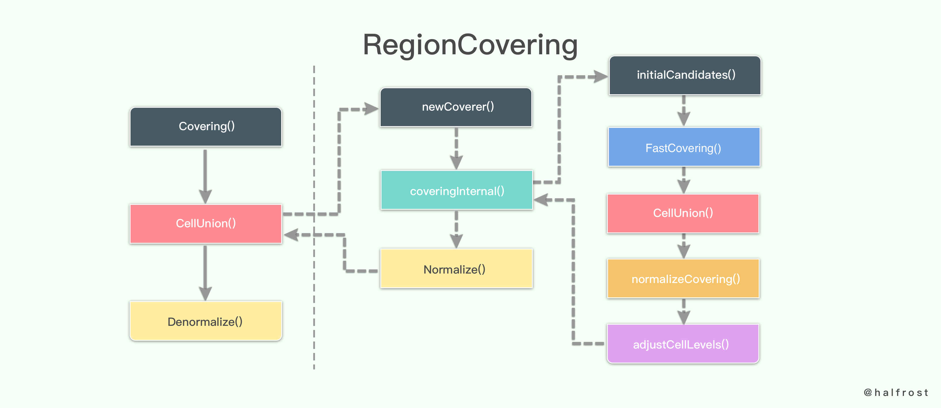
Every key implementation in the diagram above has already been analyzed. If any node is still unclear, you can scroll back up and review the relevant section.
This approximation algorithm is not optimal, but it works reasonably well in practice. The output does not always use the maximum number of Cells that satisfy the constraints, because doing so does not always produce a better approximation. For example, as mentioned above, if the region to be covered happens to lie at the intersection of three faces, the result may be much larger than the original region. In addition, MaxCells constrains both the search effort and the number of Cells in the final output.
Because this is an approximation algorithm, you should not rely on the stability of its output. In particular, the output of the covering algorithm may differ across versions of the library.
This algorithm can also generate interior covering Cells. An interior covering Cell is a Cell that is fully contained within the region. If no Cell satisfies the constraints, the set of interior covering Cells may be empty even for a non-empty region.
Note that, for performance reasons, it is wise to specify MaxLevel when computing interior covering Cells. Otherwise, for small or zero-area regions, the algorithm may spend a large amount of time subdividing Cells down to the leaf level in an attempt to find interior covering Cells that satisfy the constraints.
IV. Final Notes

This brings the spatial search series to an end. Naturally, I will close with a few reflections.
While studying and practicing spatial search, I consulted materials in physics, mathematics, and algorithms. From the perspectives of both physics and mathematics, this improved my understanding of space and time as a whole. Although my current understanding in this area may still be relatively shallow, it has improved a great deal compared with before. The goal has been achieved.
Finally, I would like to recommend two websites. These are also the questions I have been asked most often on Weibo.
The first question is: how were the S2 Cells in this article series drawn?
They actually come from an open-source website created by an individual: http://s2map.com/. I entered the CellIDs computed by my program there and displayed them. In effect, it serves as a visualization and exploration tool for S2.
The second question is: why can’t some of the code be found in the Go version?
The answer is that the Go implementation is not yet 100% complete, and for some pieces you still need to refer to the complete C++ and Java implementations. As for the C++ and Java source code, Google moved the code from its private repository to GitHub a few days ago, making it much easier to study and inspect. The official team has also organized some documentation on https://s2geometry.io/. Beginners are advised to start with the official API documentation. After reading the documentation, if you still have questions about the underlying principles, you can come back and browse this spatial search series. I hope it will be helpful to readers.
Spatial search article series:
How to Understand n-Dimensional Space and n-Dimensional Spacetime
Efficient Multidimensional Spatial Point Indexing Algorithms — Geohash and Google S2
How Is CellID Generated in Google S2?
Finding the LCA (Lowest Common Ancestor) in a Quadtree in Google S2
The Magical De Bruijn Sequence
How to Find Neighbors of a Hilbert Curve on a Quadtree?
How Does Google S2 Solve the Optimal Spatial Covering Problem?
GitHub Repo: Halfrost-Field
Follow: halfrost · GitHub