How to Understand Gradient Descent?
Because Ghost’s syntax for recognizing LaTeX differs from standard LaTeX syntax, the LaTeX formulas in the following article may appear garbled for better generality. If that happens, and if you do not mind, you can read the garble-free version of this article on the author’s Github. I will fix this garbling issue when I have time. Thank you for your understanding.
GitHub Repo: Halfrost-Field
Follow: halfrost · GitHub
Source: https://github.com/halfrost/Halfrost-Field/blob/master/contents/Machine_Learning/Gradient_descent.ipynb
I. Model Representation
Given a training set, learn a function h: X→Y such that h(x) is a “good” predictor of the corresponding value y. For historical reasons, this function h is called a hypothesis.
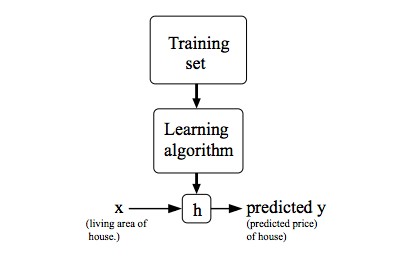
By inputting the housing area x, the learned function outputs the estimated price of the house.
II. Cost Function
The cost function is an application in linear regression. In linear regression, one problem to solve is a minimization problem.
Suppose that in univariate linear regression, given a training set, we need to find a straight line that is as close as possible to the points in that training set. Assume the equation of the line is
$$h_{\theta}(x) = \theta_{0} + \theta_{1}x$$
How should we choose $\theta_{0}$ and $\theta_{1}$ so that $h_{\theta}(x)$ is closer to the training set (x,y)?
The above problem can be transformed into finding the minimum of $$ \rm{CostFunction} = \rm{F}({\theta_{0}},{\theta_{1}}) = \frac{1}{2m}\sum_{i = 1}^{m} (h_{\theta}(x^{(i)})-y^{(i)})^2 $$, i.e., finding $$\min_{{\theta_{0}} {\theta_{1}}} \rm{F}({\theta_{0},{\theta_{1}})} $$
III. Gradient Descent
The main idea of gradient descent:
- Initialize ${\theta_{0}}$ and ${\theta_{1}}$, with ${\theta_{0}}$ = 0 and ${\theta_{1}}$ = 0
- Continuously change the values of ${\theta_{0}}$ and ${\theta_{1}}$, continuously reducing $F({\theta_{0}},{\theta_{1}})$ until it reaches the minimum value (or a local minimum).
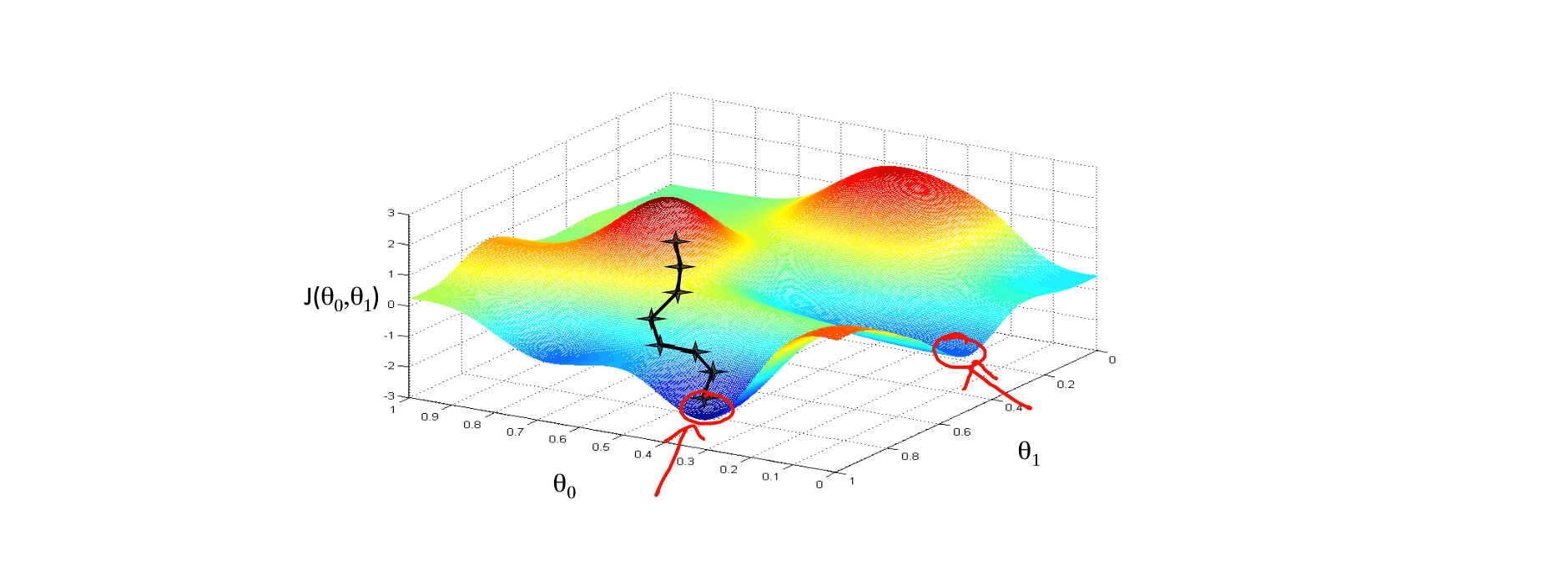
Imagine going downhill. How can you go downhill the fastest? This involves the speed of descent, namely the step size.
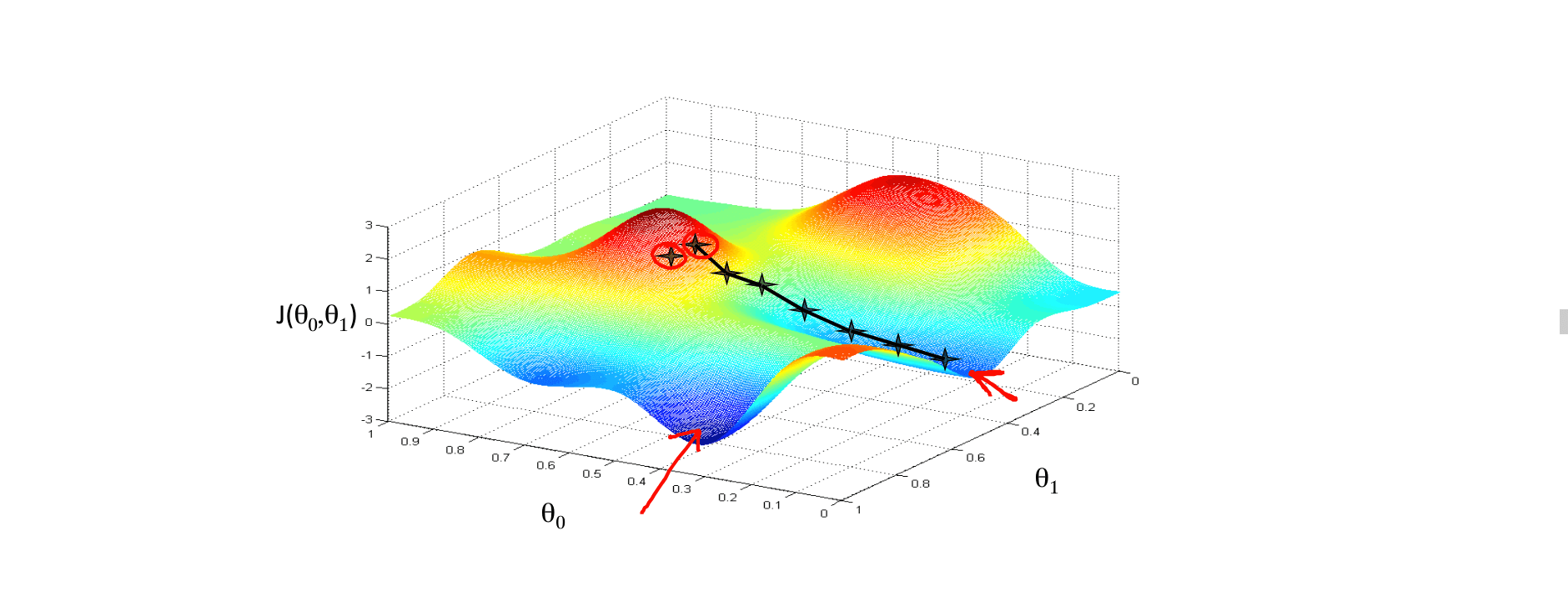
Interestingly, if you switch to a nearby point and go downhill, the optimal solution you find may be another one. This is also a characteristic of gradient descent: it will find all local optima.
The gradient descent algorithm updates continuously:
\begin{align*}
\rm{temp}0 &:= {\theta_{0}} - \alpha * \frac{\partial }{\partial {\theta_{0}}}\rm{F}({\theta_{0}},{\theta_{1}}) \
\rm{temp}1 &:= {\theta_{1}} - \alpha * \frac{\partial }{\partial {\theta_{1}}}\rm{F}({\theta_{0}},{\theta_{1}}) \
{\theta_{0}} &:= \rm{temp}0 \
{\theta_{1}} &:= \rm{temp}1 \
\end{align*}
until convergence. Note that the values of ${\theta_{0}}$ and ${\theta_{1}}$ must be **updated simultaneously**. **Remember: do not update once after computing one derivative!**
$\alpha$ is called the learning rate.
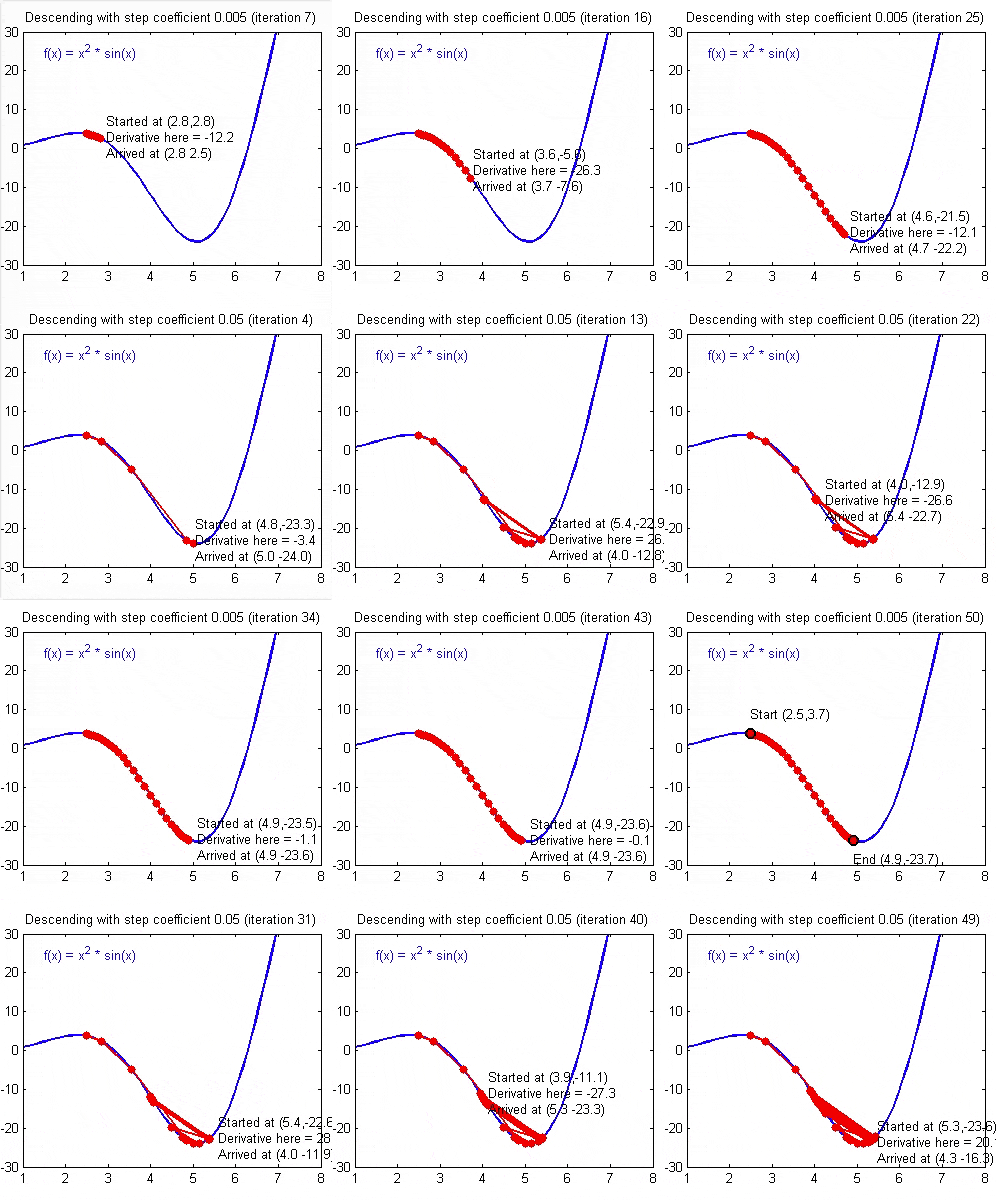
If $\alpha$ is set very small, many iterations are needed to reach the lowest point. If $\alpha$ is set very large, the algorithm may bounce back and forth and get farther and farther away from the lowest point, which can cause failure to converge, or even divergence.
When approaching the lowest point, gradient descent becomes slower and slower because $ \frac{\partial }{\partial {\theta}}$ becomes smaller and smaller.
Relationship Between Gradient and Partial Derivatives
In the gradient descent algorithm above, we have been discussing things in terms of partial derivatives. Some people may wonder: what is the relationship between partial derivatives and the gradient?
1. Derivative
If the function is univariate, then the partial derivative reduces to the ordinary derivative.
$$ f^{'}(x_{0}) = \lim_{\Delta x\rightarrow 0} \frac{\Delta y}{\Delta x} = \lim_{\Delta x\rightarrow 0} \frac{f(x_{0} + \Delta x) - f(x_{0}))}{\Delta x} $$
The geometric meaning of the derivative is the slope of the tangent line at that point, and its physical meaning is the (instantaneous) rate of change of the function at that point.
2. Partial Derivative
Now let’s look at the definition of partial derivatives:
$$ f_{x}(x_{0},y_{0}) = \lim_{\Delta x \rightarrow 0} \frac{f(x_{0} + \Delta x , y_{0}) - f(x_{0},y_{0})}{\Delta x} $$ $$ f_{y}(x_{0},y_{0}) = \lim_{\Delta y \rightarrow 0} \frac{f(x_{0} , y_{0} + \Delta y) - f(x_{0},y_{0})}{\Delta y} $$
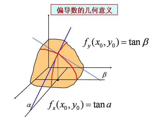
The geometric meaning of a partial derivative is also the slope of a tangent line. However, because we are on a surface, at a point on that surface, there is a plane tangent to the surface curve, which means there are infinitely many tangent lines. Here we are interested in two tangent lines: one perpendicular to the y-axis (parallel to the xOz plane), and the other perpendicular to the x-axis (parallel to the yOz plane). The slopes corresponding to these two tangent lines are the partial derivative with respect to X and the partial derivative with respect to Y.
The partial derivative of a multivariable function is its derivative with respect to one of the variables while keeping the other variables constant (as opposed to the total derivative, in which all variables are allowed to vary).
The physical meaning of a partial derivative is the rate of change of the function along the positive direction of a coordinate axis.
3. Directional Derivative
Before discussing the gradient, we should not omit the directional derivative. A partial derivative is a derivative in two specific directions, but a derivative also exists in any arbitrary direction. This introduces the concept of the directional derivative.
Suppose the function u = u(x,y) is defined in some neighborhood $ U \subset R^{2}$ of the point $p_{0}(x_{0},y_{0})$, and L is a ray starting from the point $p_{0}$. Let $p(x_{0},y_{0})$ be any point on L and inside U, and let $t = \sqrt{(\Delta x)^{2} +(\Delta y)^{2} }$ denote the distance between $p$ and $p_{0}$. If the limit:
$$ \left.\begin{matrix} \frac{\partial f}{\partial l} \end{matrix}\right|_{(x_{0},y_{0})} = \lim_{t \rightarrow 0^{+}} \frac{f(x_{0} + tcos \alpha , y_{0} + tcos \beta) - f(x_{0},y_{0})}{t} $$
exists, then this limit is called the directional derivative of the function u = u(x,y) at the point $p_{0}$ along the direction L, denoted by $ \left.\begin{matrix} \frac{\partial f}{\partial l} \end{matrix}\right|_{(x_{0},y_{0})}$.
The directional derivative is a generalization of the concept of partial derivatives. Partial derivatives study the rate of change in specified directions (the coordinate-axis directions); with directional derivatives, the specified direction can be arbitrary.
If the function u = u(x,y) is differentiable at the point $p_{0}(x_{0},y_{0})$, then the directional derivative of the function at that point along any direction L exists, and
$$ \left.\begin{matrix} \frac{\partial f}{\partial l} \end{matrix}\right|_{(x_{0},y_{0})} = f_{x}(x_{0},y_{0})cos \alpha + f_{y}(x_{0},y_{0})cos \beta $$
where $cos \alpha $ and $cos \beta$ are the direction cosines of direction L.
The directional derivative of a scalar field at a point along a certain vector direction describes the instantaneous rate of change of the scalar field near that point as it varies along that vector direction. This vector direction can be any direction.
The physical meaning of the directional derivative is the rate of change of the function at a point along a specific direction.
4. Gradient
Finally, let’s talk about the gradient. The definition of the gradient is:
In the case of a function of two variables, suppose the function $f(x,y)$ has continuous first-order partial derivatives in the planar region D. Then for every point $P_{0}(x_{0},y_{0}) \in D $, a vector can be defined:
$$ f_{x}(x_{0},y_{0}) \vec{i} + f_{y}(x_{0},y_{0}) \vec{j} $$
This vector is called the gradient of the function $f(x,y)$ at the point $p_{0}(x_{0},y_{0})$, denoted by $ \textbf{grad};;f(x_{0},y_{0}) $ or $ \triangledown f(x_{0},y_{0}) $, namely
$$ \textbf{grad};;f(x_{0},y_{0}) = \triangledown f(x_{0},y_{0}) = f_{x}(x_{0},y_{0}) \vec{i} + f_{y}(x_{0},y_{0}) \vec{j} $$
where $ \triangledown = \frac{\partial }{\partial x} \vec{i} + \frac{\partial }{\partial y} \vec{j} $ is called the (two-dimensional) vector differential operator, or the Nabla operator, and $ \triangledown f = \frac{\partial f}{\partial x} ;; \vec{i} + \frac{\partial f }{\partial y} ;; \vec{j} $ If the function $f(x,y)$ is differentiable at the point $p_{0}(x_{0},y_{0})$, and $\vec{e_{j}} = (cos \alpha,cos \beta)$ is the unit vector in the same direction as direction L, then:
$$
\begin{align*}
\left.\begin{matrix}
\frac{\partial f}{\partial l}
\end{matrix}\right|_{(x_{0},y_{0})} &= f_{x}(x_{0},y_{0})cos \alpha + f_{y}(x_{0},y_{0})cos \beta \
&= \textbf{grad};;f(x_{0},y_{0}) \cdot \vec{e_{j}} = \left | \textbf{grad};;f(x_{0},y_{0}) \right | cos \theta \
\end{align*}
$$
where $ \theta $ is the angle between $ \textbf{grad};;f(x_{0},y_{0}) $ and $ \vec{e_{j}} $.
- When $\theta = 0 $, $\left.\begin{matrix} \frac{\partial f}{\partial l} \end{matrix}\right|_{(x_{0},y_{0})} = \left | \textbf{grad};;f(x_{0},y_{0}) \right |$
That is, the gradient $ \textbf{grad};;f $ of the function $f(x,y)$ at a point is a vector whose direction is the direction in which the directional derivative of the function at that point attains its maximum, and whose norm is equal to that maximum directional derivative.
- When $\theta = \pi $, $\left.\begin{matrix} \frac{\partial f}{\partial l} \end{matrix}\right|_{(x_{0},y_{0})} = - \left | \textbf{grad};;f(x_{0},y_{0}) \right |$
That is, when $ \vec{e_{j}} $ is opposite to the gradient direction, the function decreases the fastest, and the directional derivative in that direction reaches its minimum value.
Therefore, gradient descent is based on this principle.
At a given point, the directional derivative of a function reaches its maximum in the direction of the gradient, and that maximum is the norm of the gradient.
In other words, along the gradient direction, the function value increases the fastest. Similarly, the minimum directional derivative is attained in the direction opposite to the gradient, and this minimum is the negative of the maximum; therefore, along the opposite direction of the gradient, the function value decreases the fastest.
| Concept | Physical meaning |
|---|---|
| Derivative $ f^{'}(x) $ | The instantaneous rate of change of the function at that point |
| Partial derivative $ \frac{\partial f(x,y) }{\partial x} $ | The rate of change of the function along a coordinate-axis direction |
| Directional derivative | The rate of change of the function at a point along a specific direction |
| Gradient $ \textbf{grad};;f(x,y) $ | The direction in which the function has the greatest rate of change at that point |
IV. Linear Regression
Gradient descent is a very commonly used algorithm. It is used not only in linear regression, but also with linear regression models and squared-error cost functions.
\begin{align*}
\frac{\partial }{\partial {\theta_{j}}}\rm{F}({\theta_{0}},{\theta_{1}}) & = \frac{\partial }{\partial {\theta_{j}}} \frac{1}{2m}\sum_{i = 1}^{m} (h_{\theta}(x^{(i)})-y^{(i)})^2\
\end{align*}
Let $ z = (h_{\theta}(x^{(i)})-y^{(i)})^2$ and $ u = h_{\theta}(x^{(i)})-y^{(i)}$; then $ z = u^2 $. Since both $f(z)$ and $f(u)$ are continuous, we have:
\begin{align*}
\frac{\partial }{\partial {\theta_{j}}}\rm{F}({\theta_{0}},{\theta_{1}}) & = \frac{\partial }{\partial {\theta_{j}}} \frac{1}{2m}\sum_{i = 1}^{m} (h_{\theta}(x^{(i)})-y^{(i)})^2\
& = \frac{1}{2m}\sum_{i = 1}^{m} \frac{\partial z }{\partial u} \frac{\partial u }{\partial {\theta_{j}}} = \frac{1}{2m} * 2 \sum_{i = 1}^{m} u \frac{\partial u }{\partial {\theta_{j}}}\
& = \frac{1}{m} \sum_{i = 1}^{m} u \frac{\partial u }{\partial {\theta_{j}}} \
\end{align*}
Expanding u as $ u = \theta_{0} + {\theta_{1}}x^{(i)}-y^{(i)}$, and setting j = 0, we get:
\begin{align*}
\frac{\partial }{\partial {\theta_{0}}}\rm{F}({\theta_{0}},{\theta_{1}}) &= \frac{1}{m} \sum_{i = 1}^{m} u \frac{\partial u }{\partial {\theta_{0}}} \
&= \frac{1}{m} \sum_{i = 1}^{m}(\theta_{0} + \theta_{1}x^{(i)} - y^{(i)}) = \frac{1}{m} \sum_{i = 1}^{m}(h_{\theta}(x^{(i)}) - y^{(i)}) \
\end{align*}
Setting j = 1, we get:
\begin{align*}
\frac{\partial }{\partial {\theta_{1}}}\rm{F}({\theta_{0}},{\theta_{1}}) &= \frac{1}{m} \sum_{i = 1}^{m} u \frac{\partial u }{\partial {\theta_{1}}}\
&= \frac{1}{m} \sum_{i = 1}^{m}(\theta_{0} + \theta_{1}x^{(i)} - y^{(i)}) * x^{(i)} = \frac{1}{m} \sum_{i = 1}^{m}(h_{\theta}(x^{(i)}) - y^{(i)}) * x^{(i)} \
\end{align*}
Gradient descent algorithm:
\begin{align*}
\rm{temp}0 &:= {\theta_{0}} - \alpha * \frac{\partial }{\partial {\theta_{0}}}\rm{F}({\theta_{0}},{\theta_{1}}) = {\theta_{0}} - \alpha * \frac{1}{m} \sum_{i = 1}^{m}(h_{\theta}(x^{(i)}) - y^{(i)}) \
\rm{temp}1 &:= {\theta_{1}} - \alpha * \frac{\partial }{\partial {\theta_{1}}}\rm{F}({\theta_{0}},{\theta_{1}}) = {\theta_{1}} - \alpha * \frac{1}{m} \sum_{i = 1}^{m}(h_{\theta}(x^{(i)}) - y^{(i)}) * x^{(i)} \
{\theta_{0}} &:= \rm{temp}0 \
{\theta_{1}} &:= \rm{temp}1 \
\end{align*}
Of course, besides using the iterative gradient descent algorithm, there are other methods for computing the minimum of the cost function, such as the normal equation method from linear algebra. However, comparing the two, gradient descent is better suited to larger datasets.
For example, after repeatedly updating the parameters with gradient descent, the curve obtained from linear regression will fit the original dataset increasingly well.
import numpy as np
x_train = np.array([[2.5], [3.5], [6.3], [9.9], [9.91], [8.02],
                    [4.5], [5.5], [6.23], [7.923], [2.941], [5.02],
                    [6.34], [7.543], [7.546], [8.744], [9.674], [9.643],
                    [5.33], [5.31], [6.78], [1.01], [9.68],
                    [9.99], [3.54], [6.89], [10.9]], dtype=np.float32)

y_train = np.array([[3.34], [3.86], [5.63], [7.78], [10.6453], [8.43],
                    [4.75], [5.345], [6.546], [7.5754], [2.35654], [5.43646],
                    [6.6443], [7.64534], [7.546], [8.7457], [9.6464], [9.74643],
                    [6.32], [6.42], [6.1243], [1.088], [10.342],
                    [9.24], [4.22], [5.44], [9.33]], dtype=np.float32)

y_data = np.array([[2.5], [3.5], [6.3], [9.9], [9.91], [8.02],
                    [4.5], [5.5], [6.23], [7.923], [2.941], [5.02],
                    [6.34], [7.543], [7.546], [8.744], [9.674], [9.643],
                    [5.33], [5.31], [6.78], [1.01], [9.68],
                    [9.99], [3.54], [6.89], [10.9]], dtype=np.float32)
import matplotlib.pyplot as plt
%matplotlib inline
plt.plot(x_train, y_train, 'bo',label='real')
plt.plot(x_train, y_data, 'r-',label='estimated')
plt.legend()
<matplotlib.legend.Legend at 0x7fb46c217908>

Linear Regression with One Variable Test
1.
Consider the problem of predicting how well a student does in her second year of college/university, given how well she did in her first year.
Specifically, let x be equal to the number of “A” grades (including A-. A and A+ grades) that a student receives in their first year of college (freshmen year). We would like to predict the value of y, which we define as the number of “A” grades they get in their second year (sophomore year).
Here each row is one training example. Recall that in linear regression, our hypothesis is hθ(x)=θ0+θ1x, and we use m to denote the number of training examples.
For the training set given above (note that this training set may also be referenced in other questions in this quiz), what is the value of m? In the box below, please enter your answer (which should be a number between 0 and 10).
Answer: 4
2.
Consider the following training set of m=4 training examples:
x y
1 0.5
2 1
4 2
0 0
Consider the linear regression model hθ(x)=θ0+θ1x. What are the values of θ0 and θ1 that you would expect to obtain upon running gradient descent on this model? (Linear regression will be able to fit this data perfectly.)
θ0=0,θ1=0.5
θ0=1,θ1=1
θ0=0.5,θ1=0.5
θ0=1,θ1=0.5
θ0=0.5,θ1=0
Answer: θ0=0,θ1=0.5
3.
Suppose we set θ0=−1,θ1=2 in the linear regression hypothesis from Q1. What is hθ(6)?
Answer: -1 + 2*6 = 11
4.
Let f be some function so that f(θ0,θ1) outputs a number. For this problem, f is some arbitrary/unknown smooth function (not necessarily the cost function of linear regression, so f may have local optima). Suppose we use gradient descent to try to minimize f(θ0,θ1) as a function of θ0 and θ1. Which of the following statements are true? (Check all that apply.)
A. No matter how θ0 and θ1 are initialized, so long as α is sufficiently small, we can safely expect gradient descent to converge to the same solution.
B. If the first few iterations of gradient descent cause f(θ0,θ1) to increase rather than decrease, then the most likely cause is that we have set the learning rate α to too large a value.
C. If θ0 and θ1 are initialized at the global minimum, then one iteration will not change their values.
D. Setting the learning rate α to be very small is not harmful, and can only speed up the convergence of gradient descent.
Answer: B, C
5.
Suppose that for some linear regression problem (say, predicting housing prices as in the lecture), we have some training set, and for our training set we managed to find some θ0, θ1 such that J(θ0,θ1)=0.
Which of the statements below must then be true? (Check all that apply.)
A. For this to be true, we must have θ0=0 and θ1=0 so that hθ(x)=0
B. We can perfectly predict the value of y even for new examples that we have not yet seen. (e.g., we can perfectly predict prices of even new houses that we have not yet seen.)
C. For these values of θ0 and θ1 that satisfy J(θ0,θ1)=0, we have that hθ(x(i))=y(i) for every training example (x(i),y(i))
D. This is not possible: By the definition of J(θ0,θ1), it is not possible for there to exist θ0 and θ1 so that J(θ0,θ1)=0
Answer: C
GitHub Repository: Halfrost-Field
Follow: halfrost · GitHub