Derivation of the Neural Network Backpropagation Algorithm
Because Ghost blogs recognize LaTeX syntax differently from standard LaTeX syntax, some LaTeX formulas in the following article may appear garbled for better portability. If that happens and you do not mind, you can read the non-garbled version of this article on the author’s GitHub. The author will fix this rendering issue when time permits. Thank you for your understanding.
GitHub Repo: Halfrost-Field
Follow: halfrost · GitHub
Source: https://github.com/halfrost/Halfrost-Field/blob/master/contents/Machine_Learning/Neural_Networks_Learning.ipynb
I. Cost Function and Backpropagation
1. Cost Function
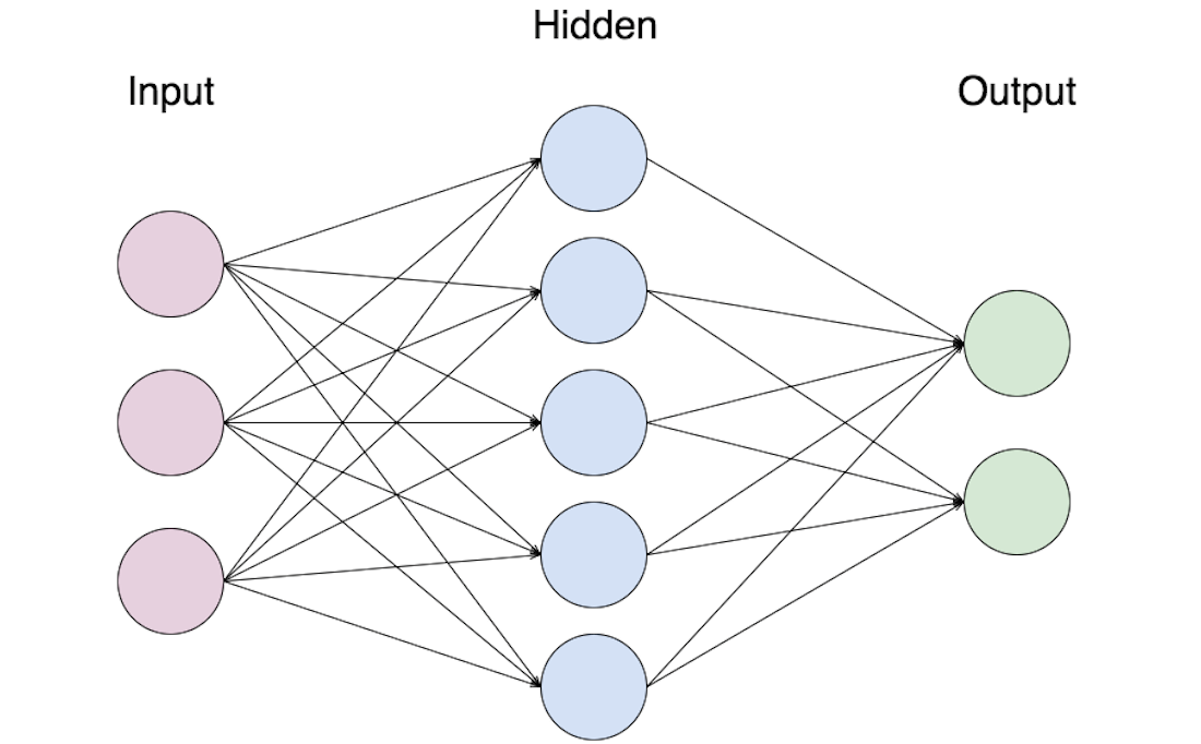
Assume the training set has m training examples, $\begin{Bmatrix} (x^{(1)},y^{(1)}),(x^{(2)},y^{(2)}), \cdots ,(x^{(m)},y^{(m)}) \end{Bmatrix}$. L denotes the total number of layers in the neural network. $S_{l}$ denotes the number of units (neurons) in the L-th layer, excluding the bias unit (constant term) in that layer. Let K be the number of units in the output layer, i.e., the number of units in the final layer.
Notation:
$z_i^{(j)}$ = the “computed value” of the $i$-th node (neuron) in the $j$-th layer
$a_i^{(j)}$ = the “activation value” of the $i$-th node (neuron) in the $j$-th layer
$\Theta^{(l)}{i,j}$ = the component in row $i$, column $j$ of the weight matrix that maps layer $l$ to layer $l+1$
$L$ = the total number of layers in the neural network (including the input layer, hidden layers, and output layer)
$s_l$ = the number of nodes (neurons) in layer $l$, excluding the bias node.
$K$ = the number of output nodes
$h{\theta}(x)_k$ = the $k$-th predicted output
$x^{(i)}$ = the feature vector of the $i$-th example
$x^{(i)}_k$ = the $k$-th feature value of the $i$-th example
$y^{(i)}$ = the actual result vector of the $i$-th example
$y^{(i)}_k$ = the $k$-th component of the result vector of the $i$-th example
The cost function for logistic regression discussed earlier is as follows:
$$
\begin{align*}
\rm{CostFunction} = \rm{F}({\theta}) &= -\frac{1}{m}\left [ \sum_{i=1}^{m} y^{(i)}logh_{\theta}(x^{(i)}) + (1-y^{(i)})log(1-h_{\theta}(x^{(i)})) \right ] +\frac{\lambda}{2m} \sum_{j=1}^{n}\theta_{j}^{2} \
\end{align*}
$$
Extending this to neural networks:
$$
\begin{align*}
\rm{CostFunction} = \rm{F}({\Theta}) &= -\frac{1}{m}\left [ \sum_{i=1}^{m} \sum_{k=1}^{K} y^{(i)}_{k} log(h_{\Theta}(x^{(i)}))_{k} + (1-y^{(i)}_{k})log(1-(h_{\Theta}(x^{(i)}))_{k}) \right ] +\frac{\lambda}{2m} \sum_{l=1}^{L-1} \sum_{i=1}^{S_{l}}\sum_{j=1}^{S_{l} +1}(\Theta_{j,i}^{(l)})^{2} \
h_{\Theta}(x) &\in \mathbb{R}^{K} ;;;;;;;;; (h_{\Theta}(x))_{i} = i^{th} ;;output \
\end{align*}
$$
$h_{\Theta}(x)$ is a K-dimensional vector, and $ i $ denotes selecting the i-th element from the neural network’s output vector.
Compared with the cost function for logistic regression, the neural network cost function has an additional $ \sum_{k=1}^{K} $ in the summation of the first term. Since K represents the number of units in the final layer, this is summing the cost functions for k output-layer units.
The latter term is the regularization term. The regularization term for a neural network looks quite complex, but it is essentially just summing the $ (\Theta_{j,i}^{(l)})^{2} $ term over all values of i, j, and l. As in logistic regression, we exclude the terms corresponding to the bias values, because we do not sum over them; that is, we do not sum the $ (\Theta_{j,0}^{(l)})^{2} ;;;;(i=0) $ terms.
2. Backpropagation Algorithm
Let $ \delta_{j}^{(l)} $ denote the error of the $j$-th node in layer $l$.
Backpropagation starts from the last layer and proceeds backward:
$$
\begin{align*}
\delta_{j}^{(L)} &= a_{j}^{(L)} - y_{j} \
&=(h_{\theta}(x))_{j} - y_{j} \
\end{align*}
$$
Compute a few steps backward:
$$
\begin{align*}
\delta^{(3)} &= (\Theta^{(3)})^{T}\delta^{(4)} . * g^{'}(z^{(3)}) \
\delta^{(2)} &= (\Theta^{(2)})^{T}\delta^{(3)} . * g^{'}(z^{(2)}) \
\end{align*}
$$
Derivative of the logistic function (Sigmoid function):
$$
\begin{align*}
\sigma(x)'&=\left(\frac{1}{1+e^{-x}}\right)‘=\frac{-(1+e^{-x})'}{(1+e^{-x})^2}=\frac{-1’-(e^{-x})'}{(1+e^{-x})^2}=\frac{0-(-x)'(e^{-x})}{(1+e^{-x})^2}=\frac{-(-1)(e^{-x})}{(1+e^{-x})^2}=\frac{e^{-x}}{(1+e^{-x})^2} \newline &=\left(\frac{1}{1+e^{-x}}\right)\left(\frac{e^{-x}}{1+e^{-x}}\right)=\sigma(x)\left(\frac{+1-1 + e^{-x}}{1+e^{-x}}\right)=\sigma(x)\left(\frac{1 + e^{-x}}{1+e^{-x}} - \frac{1}{1+e^{-x}}\right)\
&=\sigma(x)(1 - \sigma(x))\
\end{align*}
$$
We can compute $g^{'}(z^{(3)}) = a^{(3)} . * (1-a^{(3)})$ and $g^{'}(z^{(2)}) = a^{(2)} . * (1-a^{(2)})$.
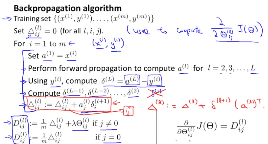
Thus, the steps of the backpropagation algorithm can be given as follows:
First, we have a training set $\begin{Bmatrix} (x^{(1)},y^{(1)}),(x^{(2)},y^{(2)}), \cdots ,(x^{(m)},y^{(m)}) \end{Bmatrix}$. For every $(l,i,j)$, set the initial value $\Delta^{(l)}_{i,j} := 0$; that is, the initial matrix is an all-zero matrix.
For the $1-m$ training set, start the following training steps:
(1) Forward Propagation
Set $ a^{(1)} := x^{(t)} $, and compute the activations $a^{(l)}$ for each layer according to the forward propagation procedure.
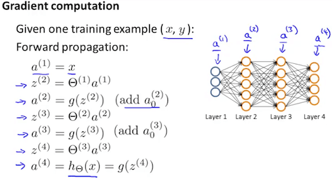
(2) Compute the Error
Using $y^{(t)}$, compute $\delta^{(L)} = a^{(L)} - y^{t}$
Here, $L$ is the total number of layers, and $a^{(L)}$ is the vector output by the activation units in the final layer. Therefore, the “error value” of the final layer is simply the difference between the actual result in the final layer and the correct output in y. To obtain the delta values for the layers before the final layer, we can use the equation in the next step and proceed from right to left:
(3) Backpropagation
Compute $\delta^{(L-1)},\delta^{(L-2)},\cdots,\delta^{(2)}$ using $\delta^{(l)} = ((\Theta^{(l)})^{(T)}\delta^{(l+1)}).* a^{(l)} .*(1-a^{(l)})$, thereby computing the error for the neural nodes in each layer.
(4) Compute Partial Derivatives
Finally, use $\Delta^{(l)}{i,j} := \Delta^{(l)}{i,j} + a_{j}^{(l)}\delta_{i}^{(l+1)}$, or in vector form, $\Delta^{(l)} := \Delta^{(l)} + \delta^{(l+1)}(a^{(l)})^{T}$.
$$ \frac{\partial }{\partial \Theta_{i,j}^{(l)} }F(\Theta) = D_{i,j}^{(l)} := \left{\begin{matrix} \frac{1}{m} \left( \Delta_{i,j}^{(l)} + \lambda\Theta_{i,j}^{(l)} \right) ;;;;;;;; j\neq 0\ \frac{1}{m}\Delta_{i,j}^{(l)} ;;;;;;;;;;;;;;;;;;;;;;; j = 0 \end{matrix}\right.$$
(5) Update the Matrices
Update the weight matrices $\Theta^{(l)}$ for each layer, where $\alpha$ is the learning rate:
$$\Theta^{(l)} = \Theta^{(l)} - \alpha D^{(l)}$$
II. Derivation
1. Objective
Find $\min_\Theta F(\Theta)$
2. Approach
Similar to gradient descent, after an initial value is given, compute the computed values and activation values of all nodes, then continuously adjust the parameter values (weights) according to changes in the cost function, ultimately approaching the optimal result and minimizing the value of the cost function.
3. Derivation Process
To implement the above approach, we must first compute the partial derivative of the cost function:
$$\dfrac{\partial}{\partial \Theta_{i,j}^{(l)}}F(\Theta)$$ This partial derivative is not easy to compute. To make the derivation easier, we assume there is only one sample ($m=1$, so the outer summation in the cost function can be ignored), and we drop the regularization term. We then handle it in two cases.
Case 1 Hidden layer → output layer
We know that:
$$
\begin{align*}
h_\Theta(x) &= a^{(j+1)} = g(z^{(j+1)}) \
z^{(j)} &= \Theta^{(j-1)}a^{(j-1)} \
\end{align*}
$$
In addition, the output layer is layer $L$.
Therefore:
$$\dfrac{\partial}{\partial \Theta_{i,j}^{(L)}}F(\Theta) = \dfrac{\partial F(\Theta)}{\partial h_{\Theta}(x)_i} \dfrac{\partial h_{\Theta}(x)_i}{\partial z_i^{(L)}} \dfrac{\partial z_i^{(L)}}{\partial \Theta_{i,j}^{(L)}} = \dfrac{\partial F(\Theta)}{\partial a_i^{(L)}} \dfrac{\partial a_i^{(L)}}{\partial z_i^{(L)}} \dfrac{\partial z_i^{(L)}}{\partial \Theta_{i,j}^{(L)}}$$
where:
$$
\begin{align*}
\dfrac{\partial F(\Theta)}{\partial a_i^{(L)}} &= \dfrac{a_i^{(L)} - y_i}{(1 - a_i^{(L)})a_i^{(L)}} \
\dfrac{\partial a_i^{(L)}}{\partial z_i^{(L)}} &= \dfrac{\partial g(z_i^{(L)})}{\partial z_i^{(L)}} = \dfrac{e^{z_i^{(L)}}}{(e^{z_i^{(L)}}+1)^2} = a_i^{(L)} (1 - a_i^{(L)}) \
\dfrac{\partial z_i^{(L)}}{\partial \Theta_{i,j}^{(L)}} &= \dfrac{\partial ( \sum_{k=0}^{s_{(L-1)}}; \Theta_{i,k}^{(L)} a_k^{(L-1)})}{\partial \Theta_{i,j}^{(L)}} = a_j^{(L-1)} \
\end{align*}
$$
Putting it all together:
$$
\begin{split}
\dfrac{\partial}{\partial \Theta_{i,j}^{(L)}}F(\Theta)
=& \dfrac{\partial F(\Theta)}{\partial a_i^{(L)}} \dfrac{\partial a_i^{(L)}}{\partial z_i^{(L)}} \dfrac{\partial z_i^{(L)}}{\partial \Theta_{i,j}^{(L)}} \newline
=& \dfrac{a_i^{(L)} - y_i}{(1 - a_i^{(L)})a_i^{(L)}} a_i^{(L)} (1 - a_i^{(L)}) a_j^{(L-1)} \newline
=& (a_i^{(L)} - y_i)a_j^{(L-1)}
\end{split}
$$
Case 2 Hidden layer / input layer → hidden layer
Because $a^{(1)}=x$, the input layer and hidden layers can be treated in the same way.
$$\dfrac{\partial}{\partial \Theta_{i,j}^{(l)}}F(\Theta) =\dfrac{\partial F(\Theta)}{\partial a_i^{(l)}} \dfrac{\partial a_i^{(l)}}{\partial z_i^{(l)}} \dfrac{\partial z_i^{(l)}}{\partial \Theta_{i,j}^{(l)}}\ (l = 1, 2, …, L-1)$$
The latter two partial derivatives can be easily inferred from the preceding results:
$$
\begin{align*}
\dfrac{\partial a_i^{(l)}}{\partial z_i^{(l)}} &= \dfrac{e^{z_i^{(l)}}}{(e^{z_i^{(l)}}+1)^2} = a_i^{(l)} (1 - a_i^{(l)}) \
\dfrac{\partial z_i^{(l)}}{\partial \Theta_{i,j}^{(l)}} &= a_j^{(l-1)} \
\end{align*}
$$
The first partial derivative is difficult to solve, or rather cannot be solved directly. We can obtain a recurrence relation:
$$\dfrac{\partial F(\Theta)}{\partial a_i^{(l)}} = \sum_{k=1}^{s_{(l+1)}} \Bigg[\dfrac{\partial F(\Theta)}{\partial a_k^{(l+1)}} \dfrac{\partial a_k^{(l+1)}}{\partial z_k^{(l+1)}} \dfrac{\partial z_k^{(l+1)}}{\partial a_i^{(l)}}\Bigg]$$
Because the activation value of this layer is related to every node in the next layer, applying the chain rule requires differentiating each of them, which gives the summation in the expression above.
In the recurrence relation, the first part is the recursive term, and the latter two parts are likewise easy to compute:
$$
\begin{align*}
\dfrac{\partial a_k^{(l+1)}}{\partial z_{k}^{(l+1)}} &= \dfrac{e^{z_{k}^{(l+1)}}}{(e^{z_{k}^{(l+1)}}+1)^2} = a_k^{(l+1)} (1 - a_k^{(l+1)}) \
\dfrac{\partial z_k^{(l+1)}}{\partial a_i^{(l)}} &= \dfrac{\partial ( \sum_{j=0}^{s_l} \Theta_{k,j}^{(l+1)} a_j^{(l)})}{\partial a_i^{(l)}} = \Theta_{k,i}^{(l+1)} \
\end{align*}
$$
Therefore, the recurrence relation is:
$$
\begin{split}
\dfrac{\partial F(\Theta)}{\partial a_i^{(l)}}
=& \sum_{k=1}^{s_{(l+1)}} \Bigg[\dfrac{\partial F(\Theta)}{\partial a_k^{(l+1)}} \dfrac{\partial a_k^{(l+1)}}{\partial z_k^{(l+1)}} \dfrac{\partial z_k^{(l+1)}}{\partial a_i^{(l)}}\Bigg] \newline
=& \sum_{k=1}^{s_{(l+1)}} \Bigg[ \dfrac{\partial F(\Theta)}{\partial a_k^{(l+1)}} \dfrac{\partial a_k^{(l+1)}}{\partial z_k^{(l+1)}} \Theta_{k,i}^{(l+1)} \Bigg] \newline
=& \sum_{k=1}^{s_{(l+1)}} \Bigg[ \dfrac{\partial F(\Theta)}{\partial a_k^{(l+1)}} a_k^{(l+1)} (1 - a_k^{(l+1)}) \Theta_{k,i}^{(l+1)} \Bigg]
\end{split}
$$
To simplify the expression, define the error of node $i$ in layer $l$ as:
$$\begin{split}
\delta^{(l)}i
=& \dfrac{\partial F(\Theta)}{\partial a_i^{(l)}} \dfrac{\partial a_i^{(l)}}{\partial z_i^{(l)}} \newline
=& \dfrac{\partial F(\Theta)}{\partial a_i^{(l)}} a_i^{(l)} (1 - a_i^{(l)}) \newline
=& \sum{k=1}^{s_{(l+1)}} \Bigg[ \dfrac{\partial F(\Theta)}{\partial a_k^{(l+1)}} \dfrac{\partial a_k^{(l+1)}}{\partial z_k^{(l+1)}} \Theta_{k,i}^{(l+1)} \Bigg] a_i^{(l)} (1 - a_i^{(l)}) \newline
=& \sum_{k=1}^{s_{(l+1)}} \Big[\delta^{(l+1)}_k \Theta_{k,i}^{(l+1)} \Big] a_i^{(l)} (1 - a_i^{(l)})
\end{split}$$
Thus, the error in Case 1 is:
$$\begin{split}
\delta^{(L)}_i
=& \dfrac{\partial F(\Theta)}{\partial a_i^{(L)}} \dfrac{\partial a_i^{(L)}}{\partial z_i^{(L)}} \newline
=& \dfrac{a_i^{(L)} - y_i}{(1 - a_i^{(L)})a_i^{(L)}} a_i^{(L)} (1 - a_i^{(L)}) \newline
=& a_i^{(L)} - y_i
\end{split}$$
The final partial derivative of the cost function is:
$$\begin{split}
\dfrac{\partial}{\partial \Theta_{i,j}^{(l)}}F(\Theta)
=& \dfrac{\partial F(\Theta)}{\partial a_i^{(l)}} \dfrac{\partial a_i^{(l)}}{\partial z_i^{(l)}} \dfrac{\partial z_i^{(l)}}{\partial \Theta_{i,j}^{(l)}} \newline
=& \delta^{(l)}_i \dfrac{\partial z_i^{(l)}}{\partial \Theta_{i,j}^{(l)}} \newline
=& \delta^{(l)}_i a_j^{(l-1)}
\end{split}$$
We can see that after introducing the error term $\delta^{(l)}_i$, this formula applies to both Case 1 and Case 2.
As shown above, the partial derivative of the cost function for the current layer depends on the computation results of the following layer. This is why the algorithm is called the “backpropagation algorithm”.
4. Summary of Algorithm Formulas
- Output-layer error
$$\delta^{(L)}_i = a_i^{(L)} - y_i$$
- Hidden-layer error (computed by backpropagation)
$$\delta^{(l)}i = \sum{k=1}^{s_{(l+1)}} \Big[\delta^{(l+1)}_k \Theta_{k,i}^{(l+1)} \Big] a_i^{(l)} (1 - a_i^{(l)})$$
- Partial derivative of the cost function (general form)
$$\dfrac{\partial}{\partial \Theta_{i,j}^{(l)}}F(\Theta) = \delta^{(l)}_i a_j^{(l-1)}$$
III. Backpropagation Algorithm Process
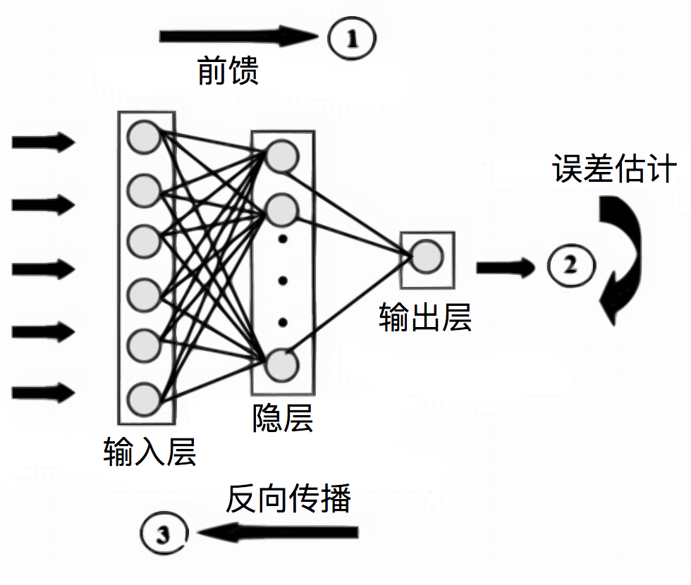
With the derivation above, we can describe the algorithm’s concrete workflow:
- Input: provide the input sample data and initialize the weight parameters (it is recommended to generate small random values).
- Feedforward: compute the node values ($z^{(l)}=\Theta^{(l-1)}a^{(l-1)}$) and activations ($a^{(l)}=g(z^{(l)})$) for each layer ($l=2, 3, …, L$).
- Output-layer error: compute the output-layer error \delta^{(L)} (see the formula above).
- Backpropagate the error: compute the error $\delta^{(l)}$ for each layer ($l=L-1, L-2, …, 2$) (see the formula above).
- Output: obtain the gradient of the cost function, $\nabla F(\Theta)$ (refer to the partial-derivative formula above).
The backpropagation algorithm gives us the gradient of the cost function, so we can train the neural network using gradient descent.
$$\Theta := \Theta - \alpha \nabla F(\Theta)$$
$\alpha $ is the learning rate.
IV. Backpropagation Algorithm Implementation
Take a 3-layer neural network as an example: one input layer, one hidden layer, and one output layer.
- X is the sample feature matrix of size number of samples ∗ number of features
- Y is the sample class (label/result) matrix of size number of samples ∗ number of output nodes
- Theta1 is the weight matrix from the input layer → hidden layer
- Theta2 is the weight matrix from the hidden layer → output layer
- m is the number of samples
- K is the number of output-layer nodes
- H is the number of hidden-layer nodes
- The sigmoid function is the logistic function (S-shaped function, Sigmoid function)
- The sigmoidGradient function is the derivative of the Sigmoid function
- The code implementation includes regularization to avoid overfitting.
1. Feedforward Phase
Compute the node values and activations layer by layer.
a1 = X;
z2 = [ones(m, 1), a1] * Theta1';
a2 = sigmoid(z2);
z3 = [ones(m, 1), a2] * Theta2';
a3 = sigmoid(z3);
2. Cost Function
For the regularization term, note that the cost function does not penalize the bias parameter, i.e., $\Theta_{i,0}$ (represented in code as $Theta(:,1)$).
F = 1 / m * sum((-log(a3) .* Y - log(1 .- a3) .* (1 - Y))(:)) + ... # cost term
 lambda / 2 / m * (sum((Theta1(:, 2:end) .^ 2)(:)) + sum((Theta2(:, 2:end) .^ 2)(:)));
 # regularization term; lambda is the regularization parameter; exclude the bias parameter Theta*(:,1)
3. Backpropagation
Compute the output-layer error and the gradient for $\Theta^{(2)}$; use backpropagation to compute the hidden-layer error and the gradient for $\Theta^{(1)}$.
Also note that bias parameters should be excluded during regularization, and remember to add a bias term $1$ to the activations.
function g = sigmoid(z)
    g = 1.0 ./ (1.0 + exp(-z));
end

function g = sigmoidGradient(z)
    g = sigmoid(z) .* (1 - sigmoid(z));
end

delta3 = a3 - Y;

Theta2_grad = 1 / m * delta3' * [ones(m, 1), a2] + ...
  lambda / m * [zeros(K, 1), Theta2(:, 2:end)]; # regularization term

delta2 = (delta3 * Theta2 .* sigmoidGradient([ones(m, 1), z2]));
delta2 = delta2(:, 2:end); # Backprop computes one extra bias error; remove it

Theta1_grad = 1 / m *  delta2' * [ones(m, 1), a1] + ...
  lambda / m * [zeros(H, 1), Theta1(:, 2:end)]; # regularization term
Recommended reading:
Principles of training multi-layer neural network using backpropagation
How can the backpropagation algorithm be explained intuitively?
GitHub Repo:Halfrost-Field
Follow: halfrost · GitHub