A First Look at Neural Networks
Because Ghost blogs recognize LaTeX with syntax that differs from standard LaTeX syntax, for better portability the LaTeX formulas in the following article may appear as garbled text. If that happens, and if you do not mind, you can read the garble-free version of this article on the author’s GitHub. The author will fix this garbling issue when time permits. Thank you for your understanding.
GitHub Repo: Halfrost-Field
Follow: halfrost · GitHub
Source: https://github.com/halfrost/Halfrost-Field/blob/master/contents/Machine_Learning/Neural_Networks_Representation.ipynb
I. Motivations
Suppose we use the logistic regression approach discussed earlier to solve the following classification problem:
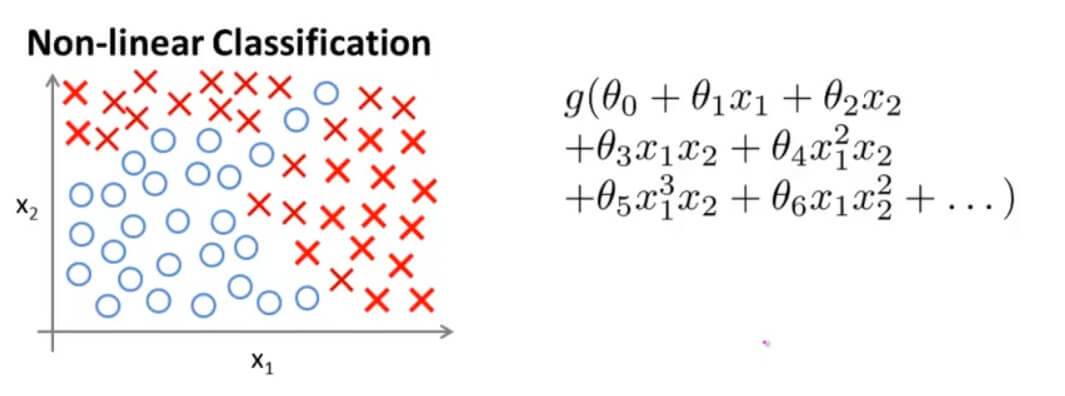
We need to construct a nonlinear logistic regression function with many terms. When there are only two features, this is still relatively simple. But what if we have 100 features? If we consider only second-order terms, the number of such terms is approximately $\frac{n^2}{2}$ . If we want to include all second-order terms, this does not look like a good approach, because there are simply too many terms and too much computation, and the final result is often prone to overfitting. Of course, we have only considered second-order terms; considering terms above second order would introduce even more.
As the number of initial features n increases, the number of these high-order polynomial terms will grow geometrically, and the feature space will expand rapidly as well. Therefore, when the number of features n is relatively large, building a classifier with this method is not a good practice.
For most machine learning problems, n is generally relatively large.
Performing linear regression on a complex dataset with many features is expensive. For example, if we classify 50 * 50 pixel black-and-white images, we already have 2500 features. If we also include all quadratic features, the complexity is $O(n^{2}/2)$, which means there would be $2500^{2}/2=3125000$ features in total. The computational cost would be very high.
Artificial neural networks are a method for applying machine learning to complex problems with many features.
II. Neural Networks
Artificial neural networks are a simplified simulation of biological neural networks. So let us start with biological neurons and then understand how neural networks work.
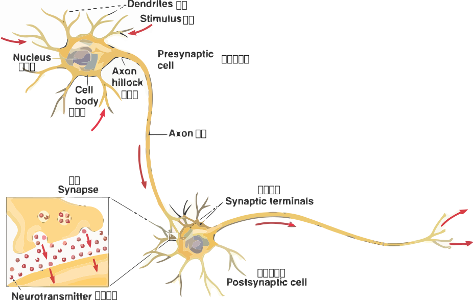
Using a simple model to simulate how a neuron works, we model the neuron as a logistic unit:
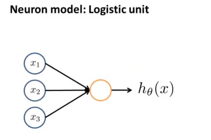
$x_{1},x_{2},x_{3}$ can be regarded as input neural dendrites, the yellow circle can be regarded as the central processor nucleus, and $h_\theta(x)$ can be regarded as the output neural axon. Since this is a logistic unit, our output function is: $h_\theta(x)=\frac{1}{1+e^{-\theta^Tx}}$ . In general, we call this an artificial neuron with an S-shaped function (logistic function) as its activation.
A neural network is essentially a collection of these neurons combined together, as shown below:
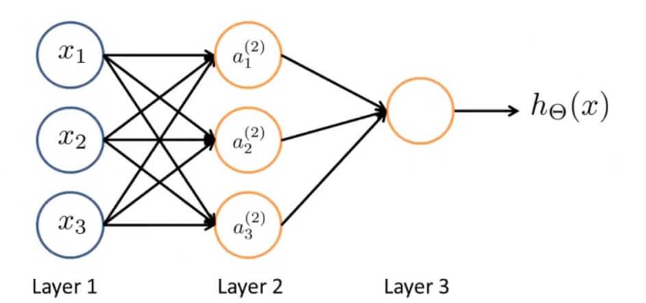
The first layer on the left, Layer1, is called the input layer. In the input layer, we feed in our features $x_{1},x_{2},x_{3}$ .
The last layer on the right is called the output layer. The output function is: $h_\Theta(x)$ .
The middle layer is called the hidden layer.
We now want to compute the value of the current neuron. In the layer preceding the one that contains the current neuron, there are many presynaptic neurons (the current neuron is the postsynaptic neuron relative to them).
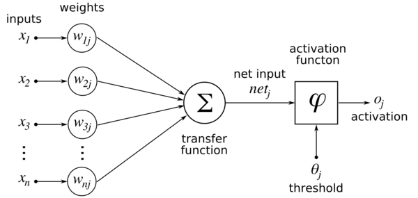
For each presynaptic neuron in the previous layer, there is an output value, which serves as the input value of the current neuron and is transmitted to the current neuron through the axon. Of course, if it is a neuron in the first layer, it receives stimuli directly from the input sample data (corresponding to $x_{i}$ in the figure).
Axons have weights (corresponding to the weights column in the figure: $w_{ij}$). We compute the weighted sum of each output value to obtain the input value of that neuron. This weighted sum corresponds to the transfer function in the figure, but the name of this function is not unambiguous. Some people call it the activation function; different people may use different names. This is only for reference here.
After obtaining the value of the neuron, we need to determine whether the neuron is activated/excited. This corresponds to the activation function in the figure, but some people also call this function the output function, while calling the preceding part the activation function and collectively referring to these two parts as the transfer function.
Several kinds of functions can be used as activation functions:
- Step function. This is the simplest and most direct form, and it is also the one commonly used when defining artificial neural networks.
- Logistic function. This is the S-shaped function (Sigmoid function), which has the advantage of being infinitely differentiable.
- Ramp function
- Gaussian function
- …
You can notice the threshold in the figure, $\theta_{j}$, namely the activation threshold. That is, only when the value of the neuron is greater than this threshold will the neuron be activated/excited and output 1; otherwise it cannot be activated and outputs 0.
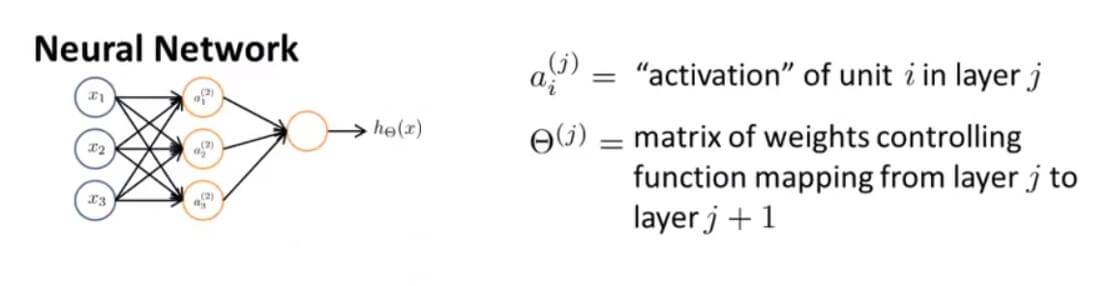
The elements in the hidden layer are denoted by $a_i^{(j)}$ . The superscript j indicates which layer it is (sometimes we do not have just a single simple layer), and the subscript i indicates which one it is: the “activation value” of the i-th node (neuron) in the j-th layer.
The neural network above can be represented simply as:
$$\begin{bmatrix} x_{0}\ x_{1}\ x_{2}\ x_{3} \end{bmatrix} \rightarrow \begin{bmatrix} a_{1}^{(2)}\ a_{2}^{(2)}\ a_{3}^{(2)} \end{bmatrix} \rightarrow h_{\theta}(x) $$
The input layer on the left has one additional bias unit (bias neuron), $x_{0}$
Use $\Theta^{(j)}$ to denote the parameters in front of the features. It is a weighted matrix that controls the size of the parameters of a layer, the weight matrix that maps layer j to layer j+1.
The neural network above can be expressed mathematically as follows:
$$
\begin{align*}
a_{1}^{(2)} &= g(\Theta_{10}^{(1)}x_{0}+\Theta_{11}^{(1)}x_{1}+\Theta_{12}^{(1)}x_{2}+\Theta_{13}^{(1)}x_{3}) \
a_{2}^{(2)} &= g(\Theta_{20}^{(1)}x_{0}+\Theta_{21}^{(1)}x_{1}+\Theta_{22}^{(1)}x_{2}+\Theta_{23}^{(1)}x_{3}) \
a_{3}^{(2)} &= g(\Theta_{30}^{(1)}x_{0}+\Theta_{31}^{(1)}x_{1}+\Theta_{32}^{(1)}x_{2}+\Theta_{33}^{(1)}x_{3}) \
h_{\Theta}(x) &= a_{1}^{(3)} = g(\Theta_{10}^{(2)}a_{0}^{(2)}+\Theta_{11}^{(2)}a_{1}^{(2)}+\Theta_{12}^{(2)}a_{2}^{(2)}+\Theta_{13}^{(2)}a_{3}^{(2)}) \
\end{align*}
$$
The $\Theta$ matrix is also referred to as the model’s weights. Here, each $g(x)$ is the sigmoid activation function, namely $g(x) = \frac{1}{1+e^{-x}}$
Vectorizing the mathematical expression of the neural network above, let:
$$
\begin{align*}
z_{1}^{(2)} &= \Theta_{10}^{(1)}x_{0}+\Theta_{11}^{(1)}x_{1}+\Theta_{12}^{(1)}x_{2}+\Theta_{13}^{(1)}x_{3} \
z_{2}^{(2)} &= \Theta_{20}^{(1)}x_{0}+\Theta_{21}^{(1)}x_{1}+\Theta_{22}^{(1)}x_{2}+\Theta_{23}^{(1)}x_{3} \
z_{3}^{(2)} &= \Theta_{30}^{(1)}x_{0}+\Theta_{31}^{(1)}x_{1}+\Theta_{32}^{(1)}x_{2}+\Theta_{33}^{(1)}x_{3} \
\vdots \
z_{k}^{(2)} &= \Theta_{k,0}^{(1)}x_{0}+\Theta_{k,1}^{(1)}x_{1}+\Theta_{k,2}^{(1)}x_{2}+\Theta_{k,3}^{(1)}x_{3} \
\end{align*}
$$
Then we can obtain:
$$
\begin{align*}
a_{1}^{(2)} &= g(z_{1}^{(2)}) \
a_{2}^{(2)} &= g(z_{2}^{(2)}) \
a_{3}^{(2)} &= g(z_{3}^{(2)}) \
\end{align*}
$$
Using vectors, this can be represented as:
$$x = \begin{bmatrix} x_{0}\ x_{1}\ x_{2}\ x_{3} \end{bmatrix},z^{(2)} = \begin{bmatrix} z_{1}^{(2)}\ z_{2}^{(2)}\ z_{3}^{(2)}\ \end{bmatrix} = \Theta^{(1)}x$$
To unify the input-output relationship between two adjacent layers, let $x=a^{(1)}$, and we can obtain:
$$
\begin{align*}
x &= \begin{bmatrix}
x_{0}\
x_{1}\
\vdots \
x_{n}
\end{bmatrix},z^{(j)} = \begin{bmatrix}
z_{1}^{(j)}\
z_{2}^{(j)}\
\vdots \
z_{3}^{(j)}\
\end{bmatrix}, \
\Rightarrow z^{(j)} &=\Theta^{(j-1)}a^{(j-1)}\
\end{align*}
$$
From this we can also derive a conclusion:
Suppose that in a network, layer j has $s_j$ units and layer j+1 has $s_{j+1}$ units. Then $\Theta^{(j)}$ controls the mapping matrix from layer j to layer j+1, and the dimensions of the matrix are: $s_{j+1} * (s_j + 1)$ . (For example: j=1 , $s_j=1$, $s_{j+1}$=1 , meaning that the first layer has only one unit and the second layer also has only one unit. Then the dimensions of the $\Theta^{(1)}$ matrix are 1 * 2, because the bias unit must be included.) Because we typically have $a_0^{(j)}=1$, we have:
$$
\begin{align*}
a^{(j)}&=g(z^{(j)})\
z^{(j+1)}&=\Theta^{(j)}a^{(j)}\
h_\Theta(x)&=a^{(j+1)}=g(z^{(j+1)})\
\end{align*}
$$
This relationship shows that the fundamental difference between neural networks and the logistic regression we learned earlier is that a neural network uses the output of the previous layer as the input to the next layer. The process of computing activations once from the input layer to the hidden layer and then to the output layer is called forward propagation.
III. Applications
1. Logical Operations
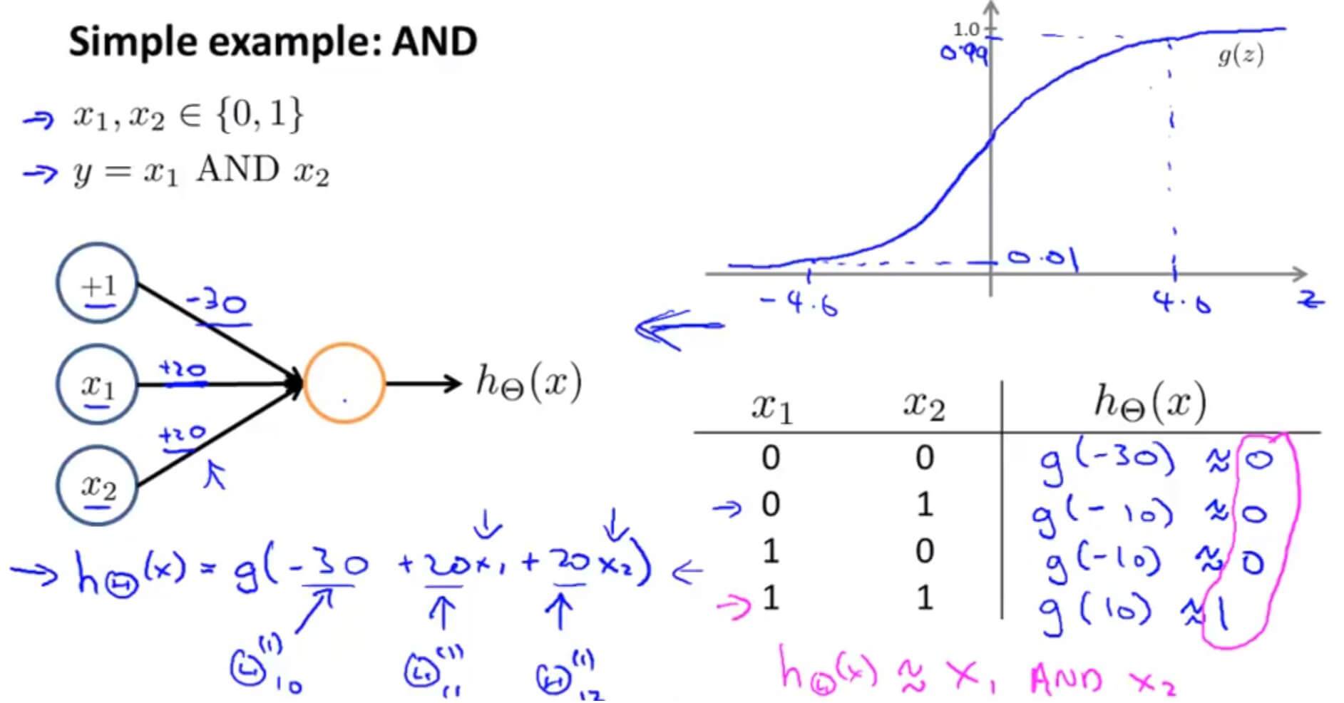
Using a neural network to perform logical AND:
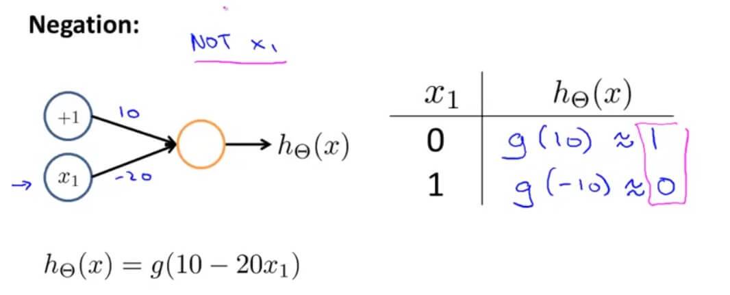
Using a neural network to perform logical NOT:
However, a single layer cannot implement XOR.
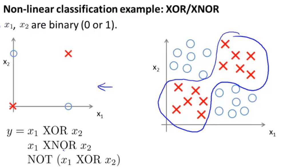
Geometrically, the XOR problem is to separate the red crosses from the blue circles. But our output function is: $h_\Theta(x)=g(\Theta_{10}^{(1)}x_0+\Theta_{11}^{(1)}x_1+\Theta_{12}^{(1)}x_2)$, which is linear. Therefore, no matter how we draw a straight line on the plot, we cannot separate the two different training sets. Since one straight line is not enough, we add one more layer to the neural network.
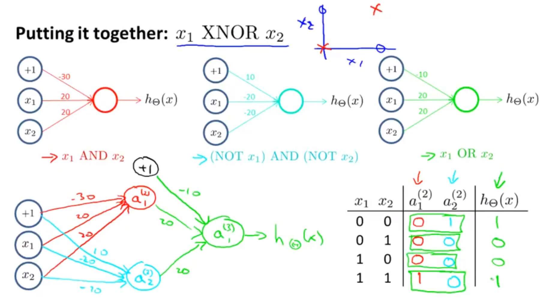
As shown above, take the first element in the second layer, $a_1^{(2)}$, as the result of the AND operation, and the second element, $a_2^{(2)}$, as the result of the NOR operation. Then use $a_1^{(2)}$ and $a_2^{(2)}$ as inputs to perform an OR operation, producing the output of the third layer. The final relationship between the result and the inputs is exactly the XOR relationship.
2. Essence
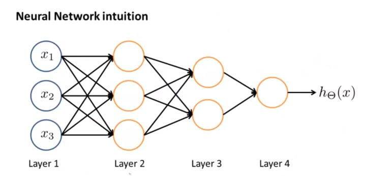
This is exactly how neural networks solve relatively complex functions. When there are many layers, we start with relatively simple inputs, apply weights and different operations, and pass them to the second layer. The third layer then uses the second layer as its input to perform more complex computations, solving the problem layer by layer.
IV. Neural Networks: Representation Quiz
1. Question 1
Which of the following statements are true? Check all that apply.
A. Suppose you have a multi-class classification problem with three classes, trained with a 3 layer network. Let a(3)1=(hΘ(x))1 be the activation of the first output unit, and similarly a(3)2=(hΘ(x))2 and a(3)3=(hΘ(x))3. Then for any input x, it must be the case that a(3)1+a(3)2+a(3)3=1.
B. The activation values of the hidden units in a neural network, with the sigmoid activation function applied at every layer, are always in the range (0, 1).
C. A two layer (one input layer, one output layer; no hidden layer) neural network can represent the XOR function.
D. Any logical function over binary-valued (0 or 1) inputs x1 and x2 can be (approximately) represented using some neural network.
Answer: B, D
B. The sigmoid function is used as the decision function at every layer, and its range is [0,1], so this is correct.
D. Any logical operation with binary inputs can be solved by a neural network, so this is correct.
C. XOR cannot be solved with a single-layer neural network.
A. Not necessarily. If the decision function is not a sigmoid function, the final results will not necessarily sum to 1.
GitHub Repo: Halfrost-Field
Follow: halfrost · GitHub