Octave Matlab Tutorial
Because Ghost Blog’s syntax for recognizing LaTeX differs from standard LaTeX syntax, the LaTeX formulas in the following article may appear garbled for better portability. If that happens, and if you don’t mind, you can read the non-garbled version of this article on the author’s Github. The author will fix this garbling issue when time permits. Thank you for your understanding.
GitHub Repo: Halfrost-Field
Follow: halfrost · GitHub
Source: https://github.com/halfrost/Halfrost-Field/blob/master/contents/Machine_Learning/Octave_Matlab_Tutorial.ipynb
I. Basic Operations
In MATLAB, % is the comment character. The basic mathematical operations are as follows:
1 + 2   %addition
5 - 6   %subtraction
7 * 4   %multiplication
9 / 3   %division
6 ^ 4   %exponentiation
log(20) %logarithmic operation
exp(30) %exponential operation
abs(-2) %absolute value operation
1. Logical Operations:
1 == 2             %Check whether equal
ans = 0            %false
--------------------------------------------------------------------------------------------
1 ~= 2             % ~= means !=, check whether not equal
ans = 1            %True
--------------------------------------------------------------------------------------------
1 && 0             %Logical AND (AND operation)
ans = 0
--------------------------------------------------------------------------------------------
1 || 0             %Logical OR(OR operation)
ans = 1
--------------------------------------------------------------------------------------------
xor(1,0)           %XOR operation
ans = 1
--------------------------------------------------------------------------------------------
2. Replace the Line-Start Prompt
PS1('>>'); %The text inside single quotes is the line-start prompt to replace
3. Variable Assignment:
a = 3        % Assign a number
a = 3;      % If you don't want it to output, you can add a semicolon(;)at the end
b = 'Hello world';   %Assign a string
--------------------------------------------------------------------------------------------
disp(a)
disp(sprintf('2 decimals :%0.2f',a))   %sprintf prints a formatted string
--------------------------------------------------------------------------------------------
format long   % Display subsequent strings with the default number of digits
a

format short  % Print fewer digits after the decimal point for subsequent strings
a
--------------------------------------------------------------------------------------------
4. Vectors and Matrices:
A = [1 2;3 4;5 6;] %create a matrix variable; the semicolon means move to the next line
A =

   1   2
   3   4
   5   6

B = [1 2 3]  %create a vector
B =

   1   2   3
--------------------------------------------------------------------------------------------

v = 1:0.1:2    % a:x:b denotes the interval [a,b], and x denotes the increment step size
v =
    1.0000    1.1000    1.2000    1.3000    1.4000    1.5000    1.6000    1.7000    1.8000    1.9000    2.0000

--------------------------------------------------------------------------------------------

ones(2,3)   %generate a 2*3 matrix whose elements are all 1
ans =
     1     1     1
     1     1     1

%If you want to generate a 2*3 matrix whose elements are all 2, of course don't use twos(2,3), but use the method below

2*ones(2,3)
ans =

   2   2   2
   2   2   2

%A similar shortcut command to ones is zeros
--------------------------------------------------------------------------------------------

zeros(1,3)  %generate a 1*3 zero matrix
ans =
     0     0     0
--------------------------------------------------------------------------------------------

rand(1,3)  %generate a 1*3 random-number matrix
ans =

   0.960762   0.089159   0.384507
--------------------------------------------------------------------------------------------
eye(2,3)   % generate a 2*3 identity matrix
ans =
     1     0     0
     0     1     0
--------------------------------------------------------------------------------------------
eye(3)     % generate a 3*3 identity matrix
ans =
     1     0     0
     0     1     0
     0     0     1
--------------------------------------------------------------------------------------------
5. Helper Functions:
help eye % Put a command name after help to display detailed usage for that command
II. Moving Data Around
1. Matrix Computation:
A = [1,2; 3,4; 5,6;];
size(A)           %Compute the matrix dimensions
ans =
     3     2
--------------------------------------------------------------------------------------------

size(A,1)         %Display the number of rows in the matrix; 1 means return rows
ans =
     3
size(A,2)         %Display the number of columns in the matrix; 2 means return columns
ans =
     2
--------------------------------------------------------------------------------------------

v = [1,2,3,4];
length(v)         % Compute the size of the vector's largest dimension; length is usually used for vectors, not matrices
ans =
     4

--------------------------------------------------------------------------------------------
2. Read and store file data:
load xxx               %xxx is the file name in the current path
load ('xxx')           %load as a string
v = xxx(1:10)          %create vector v, whose elements are data 1~10 in file xxx

--------------------------------------------------------------------------------------------

save xxx.mat V         %save the current data to a file, with variable name V
save xxx.txt V -ascii  %save the current data to an ASCII-encoded text file
3. Display commands:
pwd              %Display current path
ls               %Display folders in current path
cd 'path'        %Open this path
who              %All variables stored in current memory
whos             %Show variable names, dimensions, memory usage, and data types in more detail
clear            %Clear all variables
addpath('path')  %Add the path to the current search path
4. Matrix Indexing Operations:
A = [1,2; 3,4; 5,6;];

A(3,2)   %index the element in row 1, column 2 of the matrix
ans =
     6
--------------------------------------------------------------------------------------------

A(2,:)   %index all elements in row 2 of the matrix; the colon denotes all elements in that row or column
ans =
     3     4
A(:,2)   %index all elements in column 2 of the matrix
ans =
     2
     4
     6
--------------------------------------------------------------------------------------------

A([1 3],:)  %index all elements in rows 1 and 3 of the matrix
ans =
     1     2
     5     6
--------------------------------------------------------------------------------------------
A(:,2) = [10;11;12]  %replace the second column of A with the vector on the right
ans =
     1     10
     3     11
     5     12
--------------------------------------------------------------------------------------------

A = [A,[100;101;102]] %add a new vector as a column
A =
     1     2     100
     3     4     101
     5     6     102
--------------------------------------------------------------------------------------------

A(:)    %turn the elements of matrix A into a column vector
ans =
     1
     3
     5
     2
     4
     6
     100
     101
     102

--------------------------------------------------------------------------------------------

A = [1,2;3,4];           %merge matrices, with A on the left and B on the right
B = [4,5;6,7];
C = [A B]                %equivalent to C = [A,B]
C =
     1     2     4     5
     3     4     6     7

C = [A;B]                %merge matrices, with A on top and B below
C =
     1     2
     3     4
     4     5
     6     7

--------------------------------------------------------------------------------------------
III. Computing on Data
1. Matrix Computation:
A*B                    %Matrix multiplication
A.*B                   %Element-wise matrix multiplication (the two matrices must have the same dimensions)
A.^2                   %Square each element of the matrix
1./A                   %Take the reciprocal of each element of the matrix
log(A)                 %Take the logarithm of each element of the matrix
exp(A)                 %Raise e to the power of each element of the matrix
abs(A)                 %Get the absolute value of each element of the matrix
--------------------------------------------------------------------------------------------
A + ones(length(A),1)  %Add one to each element in A
A + 1                  %Add one to each element in A
--------------------------------------------------------------------------------------------
A'                     %Transpose of A
--------------------------------------------------------------------------------------------
A < 3                  %Compare each element in A with 3; 0 is false, 1 is true
find(A<3)              %Find all elements in A less than 3 and return their indices
[r,c] = find(A>=7)     %r and c respectively indicate the rows and columns of elements in A greater than 7
--------------------------------------------------------------------------------------------
A = magic(3)           %Generate a matrix whose rows and columns all sum to the same value, i.e., a magic square
A =
     8     1     6
     3     5     7
     4     9     2
--------------------------------------------------------------------------------------------

sum(A)                 %Sum of all elements in A
prod(A)                %Product of all elements in A
floor(A)               %Round elements in A down
ceil(A)                %Round elements in A up
rand(3)                %Generate a 3*3 random matrix
max(A,[],1)            %Maximum value in each column of A; 1 means taking values by columns of A
max(A,[],2)            %Maximum value in each row of A; 2 means taking values by rows of A
max(A)                 %Defaults to the maximum value in each column of A
max(max(A))            %Maximum value among all elements in A
max(A(:))              %Maximum value among all elements in A (first convert A to a column vector, then find the maximum)
sum(A,1)               %Sum of each column of A
sum(A,2)               %Sum of each row of A
eye(9)                 %Construct a 9*9 identity matrix
flipud(A)              %Flip the matrix vertically
pinv(A)                %Pseudo-inverse matrix of A (pseudo inverse)

--------------------------------------------------------------------------------------------
IV. Plotting Data
1. Plotting:
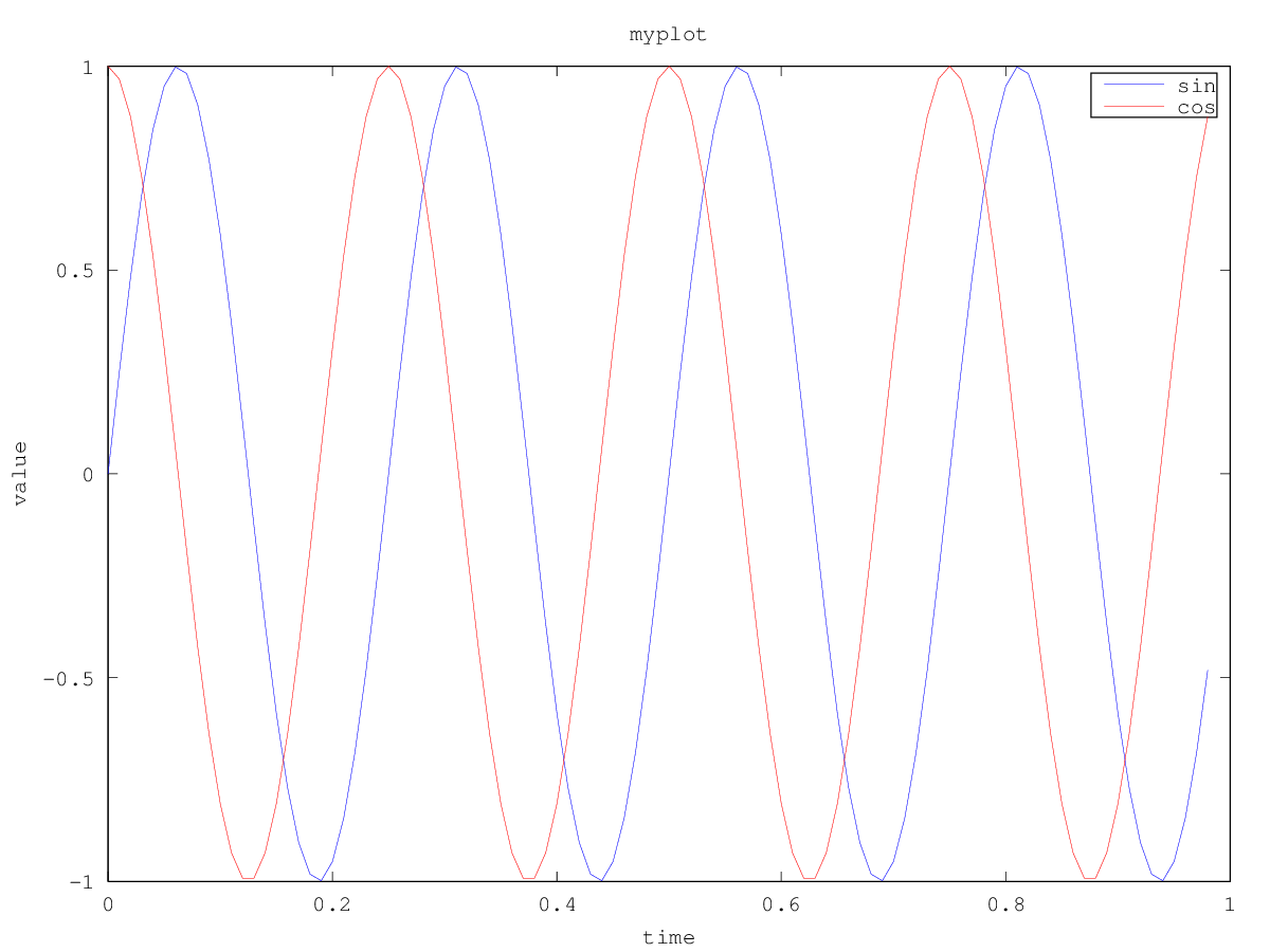
t = [0:0.01:0.98];
y1 = sin(2*pi*4*t);
y2 = cos(2*pi*4*t);
plot(t,y1);
hold on;                    %plot on the existing figure
plot(t,y2,'r');
xlabel('time');             %X-axis unit
ylabel('value');            %Y-axis unit
legend('sin','cos');        %show the two curves
title('myplot');            %add a title
print  -dpng 'myplot.png';  %export image as PNG
close                       %close
figure(1);plot(t,y1);   %Plot separately
figure(2);plot(t,y2);

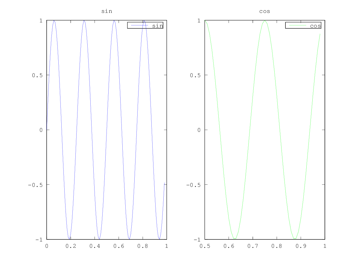
subplot(1,2,1);         %Divide the figure into a 1*2 grid, use the 1st
plot(t,y1);
subplot(1,2,2);         %Divide the figure into a 1*2 grid, use the 2nd
plot(t,y2);
axis([0.5 1 -1 1]);     %Change the axis scale: x-axis to [0.5,1], y-axis to [-1,1]
clf;                    %Clear a figure
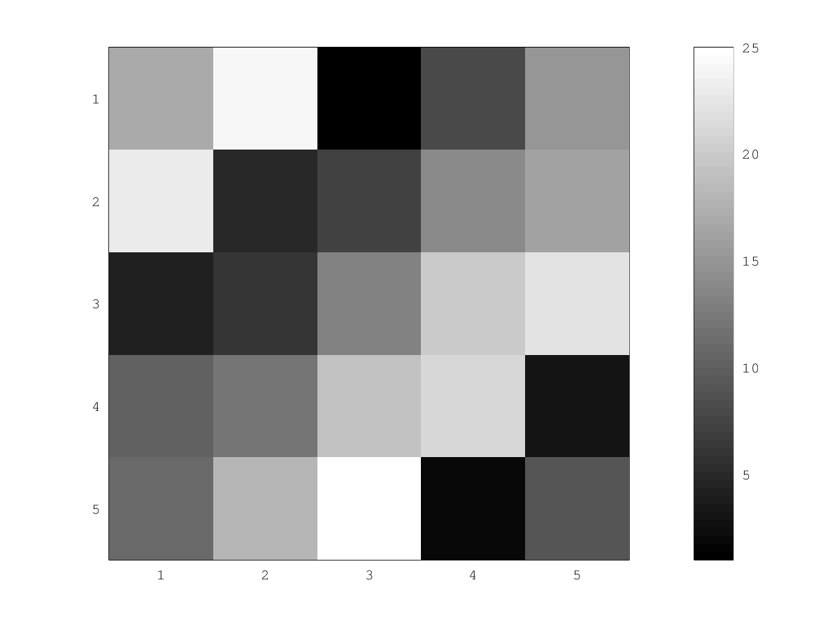
A = magic(5);
imagesc(A)                                    %Generate a colored grid plot of the matrix; different colors correspond to different values
imagesc(A), colorbar, colormap gray;         %Add a grayscale colormap and colorbar
V. Control Statements: for, while, if statement
1. Loop Statements
 v = zeros(5,1);
for i = 1:5,        %for statement
    v(i) = 2^i;
end;                %Use end as the ending marker
ans:
v =
     2
     4
     8
    16
    32

--------------------------------------------------------------------------------------------

i = 1;
while i <= 3;       %while statement
      v(i) = 100;
      i = i + 1;
end;
ans:
v =
    100
    100
    100
    16
    32


--------------------------------------------------------------------------------------------

i = 1 ;
while true,
      v(i) = 999;
      i = i + 1;
      if i==6,
         break;     %break statement
      end;
end;

--------------------------------------------------------------------------------------------


if v(1)== 1,        %if-else statement
   disp('The value is one');
elseif v(1) == 2,
   disp('The value is two');
else
   disp('The value is not one or two');
end;

--------------------------------------------------------------------------------------------
VI. Octave/Matlab Tutorial Quiz
1. Question 1
Suppose I first execute the following in Octave/Matlab:
A = [1 2; 3 4; 5 6];
B = [1 2 3; 4 5 6];
Which of the following are then valid commands? Check all that apply. (Hint: A’ denotes the transpose of A.)
A. C = A’ + B;
B. C = B * A;
C. C = A + B;
D. C = B’ * A;
Answer: A, B
Only matrices with the same dimensions can be added. The condition for multiplication is $A*B$ (columns of A = rows of B).
2. Question 2
$ Let;A= \begin{bmatrix} 16& 2 & 3 & 13\ 5& 11 & 10 & 8\ 9& 7& 6&12 \ 4& 14& 15 & 1 \end{bmatrix}$
Which of the following indexing expressions gives $ B= \begin{bmatrix} 16& 2 \ 5& 11 \ 9& 7 \ 4& 14 \end{bmatrix}$? Check all that apply.
A. B = A(:, 1:2);
B. B = A(1:4, 1:2);
C. B = A(:, 0:2);
D. B = A(0:4, 0:2);
Answer: A, B
$B = A(:, 1:2);$ First select all rows of A, then select columns 1 and 2. $B = A(1:4, 1:2);$ First select rows 1–4 of A, then select columns 1 and 2.
3. Question 3
Let A be a 10x10 matrix and x be a 10-element vector. Your friend wants to compute the product Ax and writes the following code:
v = zeros(10, 1);
for i = 1:10
  for j = 1:10
    v(i) = v(i) + A(i, j) * x(j);
  end
end
How would you vectorize this code to run without any FOR loops? Check all that apply.
A. v = A * x;
B. v = Ax;
C. v = A .* x;
D. v = sum (A * x);
Answer: A
Vectorizing the for loop
4. Question 4
Say you have two column vectors v and w, each with 7 elements (i.e., they have dimensions 7x1). Consider the following code:
z = 0;
for i = 1:7
  z = z + v(i) * w(i)
end
Which of the following vectorizations correctly compute z? Check all that apply.
A. z = sum (v .* w);
B. z = v’ * w;
C. z = v * w’;
D. z = v .* w;
Answer: A, B
The final result is a real number; from this, you can determine which option is $1*1$.
5. Question 5
In Octave/Matlab, many functions work on single numbers, vectors, and matrices. For example, the sin function when applied to a matrix will return a new matrix with the sin of each element. But you have to be careful, as certain functions have different behavior. Suppose you have an 7x7 matrix X. You want to compute the log of every element, the square of every element, add 1 to every element, and divide every element by 4. You will store the results in four matrices, A,B,C,D. One way to do so is the following code:
for i = 1:7
  for j = 1:7
    A(i, j) = log(X(i, j));
    B(i, j) = X(i, j) ^ 2;
    C(i, j) = X(i, j) + 1;
    D(i, j) = X(i, j) / 4;
  end
end
Which of the following correctly compute A,B,C, or D? Check all that apply.
A. C = X + 1;
B. D = X / 4;
C. A = log (X);
D. B = X ^ 2;
Answer: A, B, C
The last option should be $B = X. ^{} 2;$ (dot ^2)
GitHub Repo: Halfrost-Field
Follow: halfrost · GitHub