What Is Regularization?
Because Ghost blogs recognize LaTeX syntax differently from standard LaTeX syntax, the LaTeX formulas in the following article may appear garbled for better general compatibility. If that happens and you do not mind, you can read the non-garbled version of this article on the author’s Github. I will fix this rendering issue when I have time. Thank you for your understanding.
GitHub Repo: Halfrost-Field
Follow: halfrost · GitHub
Source: https://github.com/halfrost/Halfrost-Field/blob/master/contents/Machine_Learning/Regularization.ipynb
I. Solving the Problem of Overfitting
Consider the problem of predicting y from $x \in \mathbb{R}$. The leftmost plot below shows the result of fitting $y =\theta_{0}+\theta_{1}x$ to the dataset. We can see that the data is not linear, so this fit is not very good.
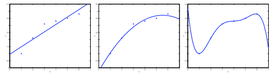
By contrast, if we add an extra feature x2 and fit $y =\theta_{0}+\theta_{1}x+\theta_{2}x^{2}$, then the data we obtain fits slightly better, as shown above.
However, adding more polynomial terms is not always better. Adding too many features is also risky: the rightmost plot is the result of fitting a fifth-degree polynomial $y =\theta_{0}+\theta_{1}x+\theta_{2}x^{2}+\theta_{3}x^{3}+\theta_{4}x^{4}+\theta_{5}x^{5} $. We can see that even though the fitted curve passes through the data perfectly, we would not consider it a good predictor. The rightmost plot above is an example of overfitting.
The rightmost plot above is also said to have high variance. If we fit a high-degree polynomial with too many features, and the hypothesis function can fit almost all of the data, then we face the problem that the set of possible functions may be too large, with too many variables. We do not have enough data to constrain it and obtain a good hypothesis function. This is overfitting.
Underfitting, or high bias, occurs when the form of our hypothesis function h has difficulty capturing the trend in the data. It is usually caused by a function that is too simple or has too few features. On the other hand, overfitting, or high variance, is caused by a hypothesis function that fits the existing data but does not predict new data well. It is usually caused by a complex function that produces many unnecessary curves and angles unrelated to the data.
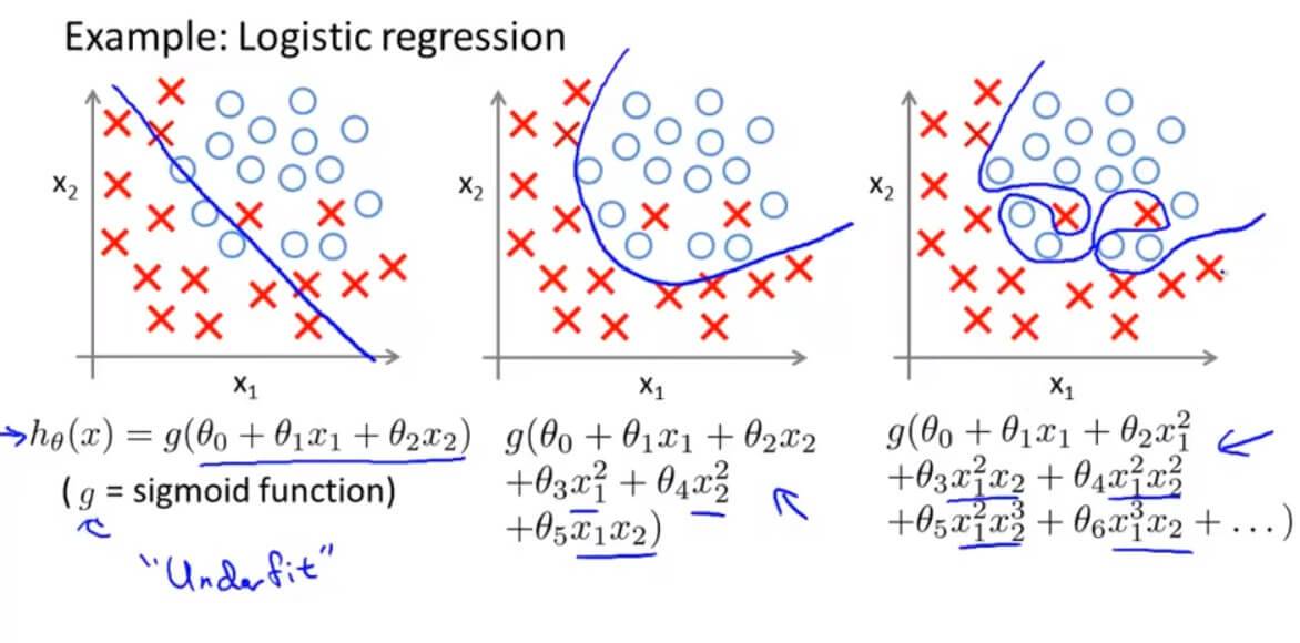
This terminology applies to both linear and logistic regression. There are two main options for solving the overfitting problem:
1. Reduce the number of features:
- Manually select which features to keep, which variables are more important, which variables should be retained, and which should be discarded.
- Use a model selection algorithm (to be covered later in the course), which automatically selects which feature variables to keep and which to discard.
The downside is that after discarding some features, we also discard some key information about the problem.
2. Regularization
- Keep all the features, but reduce the size or magnitude of the parameters $\theta_{j}$.
- When there are many features, and each feature affects the final predicted value, regularization can ensure the model works well.
The purpose of regularization is to simplify the hypothesis model as much as possible. Because when these parameters are close to 0, the simpler model has also been shown to be less prone to overfitting.
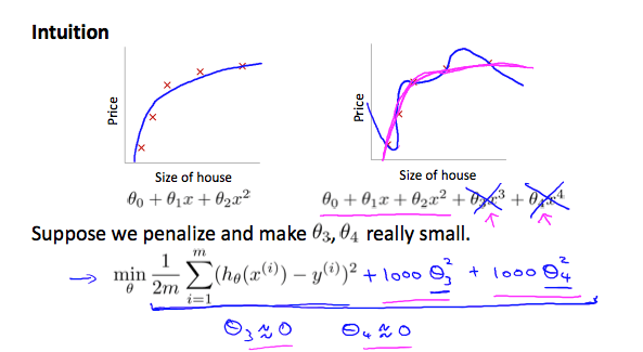
Reduce the magnitude of some features and add some “penalty” terms (to minimize the cost function, multiplying by 1000 is the penalty).
Cost function:
$$ \rm{CostFunction} = \rm{F}({\theta}) = \frac{1}{2m} \left [ \sum_{i = 1}^{m} (h_{\theta}(x^{(i)})-y^{(i)})^2 + \lambda \sum_{i = 1}^{m} \theta_{j}^{2} \right ]$$
$\lambda \sum_{i = 1}^{m} \theta_{j}^{2}$ is the regularization term, which shrinks the value of each parameter. $\lambda$ is the regularization parameter. $\lambda$ controls the trade-off between two different objectives: fitting the training set better and keeping the parameters smaller, thereby keeping the hypothesis model relatively simple and avoiding overfitting.
However, if the chosen $\lambda $ is too large, it may eliminate features too aggressively, causing all $\theta$ to be approximately 0. The final prediction function then becomes a horizontal straight line. This becomes an example of underfitting (too much bias, high bias).
II. Regularized Linear Regression
1. Gradient Descent Regularization for Linear Regression
$$\theta_{0} := \theta_{0} - \alpha \frac{1}{m} \sum_{i = 1}^{m} (h_{\theta}(x^{(i)})-y^{(i)})x_{0}^{(i)}$$
$$\theta_{j} := \theta_{j} - \alpha \left [ \left ( \frac{1}{m} \sum_{i = 1}^{m} (h_{\theta}(x^{(i)})-y^{(i)})x_{j}^{(i)}\right ) + \frac{\lambda}{m}\theta_{j} \right ] ;;;;;;;;j \in \begin{Bmatrix} 1,2,3,4, \cdots n\end{Bmatrix}$$
Simplifying the formula above gives:
$$\theta_{j} := \theta_{j}(1-\alpha \frac{\lambda}{m}) - \alpha \frac{1}{m} \sum_{i = 1}^{m} (h_{\theta}(x^{(i)})-y^{(i)})x_{j}^{(i)} ;;;;;;;;j \in \begin{Bmatrix} 1,2,3,4, \cdots n\end{Bmatrix}$$
In the formula above, $(1-\alpha \frac{\lambda}{m}) < 1$ is always less than 1 and approximately equal to 1 (0.999). Therefore, the gradient descent process multiplies the parameter by 0.999 on each update, shrinking it slightly, and then moves it a bit in the direction of the minimum point.
2. Normal Equation Regularization for Linear Regression
The conclusion for the normal equation derived earlier is:
$$\Theta = (X^{T}X)^{-1}X^{T}Y$$
After regularization, the formula above becomes:
$$\Theta = \left( X^{T}X +\lambda \begin{bmatrix} 0 & & & & \ & 1 & & & \ & & 1 & & \ & & & \ddots & \ & & & & 1 \end{bmatrix} \right) ^{-1}X^{T}Y$$
In the previous discussion, there was a prerequisite that $X^{T}X$ is a non-singular (non-degenerate) matrix, i.e. $ \left | X^{T}X \right | \neq 0 $
In the regularized formula above, as long as $\lambda > 0$, the problem of non-invertibility no longer exists. This is because the term $\left( X^{T}X +\lambda \begin{bmatrix} 0 & & & & \ & 1 & & & \ & & 1 & & \ & & & \ddots & \ & & & & 1 \end{bmatrix} \right)$ must be invertible, since it must not be a singular matrix. Therefore, regularization can also solve the non-invertibility case.
III. Regularized Logistic Regression
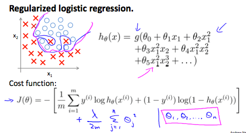
The cost function discussed earlier is:
$$
\begin{align*}
\rm{CostFunction} = \rm{F}({\theta}) &= -\frac{1}{m}\left [ \sum_{i=1}^{m} y^{(i)}logh_{\theta}(x^{(i)}) + (1-y^{(i)})log(1-h_{\theta}(x^{(i)})) \right ] \
\left( h_{\theta}(x) = \frac{1}{1+e^{-\theta^{T}x}} \right )
\end{align*}
$$
After regularization:
$$
\begin{align*}
\rm{CostFunction} = \rm{F}({\theta}) &= -\frac{1}{m}\left [ \sum_{i=1}^{m} y^{(i)}logh_{\theta}(x^{(i)}) + (1-y^{(i)})log(1-h_{\theta}(x^{(i)})) \right ] +\frac{\lambda}{2m} \sum_{j=1}^{n}\theta_{j}^{2} \
\end{align*}
$$
1. Gradient Descent Regularization for Logistic Regression
The formula is equivalent to regularization for linear regression.
$$
\begin{align*}
\theta_{0} &:= \theta_{0} - \alpha \frac{1}{m} \sum_{i = 1}^{m} (h_{\theta}(x^{(i)})-y^{(i)})x_{0}^{(i)} ;;;;;;;;;;;;;;;;;;;;;j = 1 \
\theta_{j} &:= \theta_{j}(1-\alpha \frac{\lambda}{m}) - \alpha \frac{1}{m} \sum_{i = 1}^{m} (h_{\theta}(x^{(i)})-y^{(i)})x_{j}^{(i)} ;;;;;;;;j \in \begin{Bmatrix} 1,2,3,4, \cdots n\end{Bmatrix} \
\end{align*}
$$
Although the formula is exactly the same as in linear regression, the meaning of $h_{\theta}(x)$ is different here. In logistic regression:
$$h_{\theta}(x) = \frac{1}{1+e^{-\theta^{T}x}}$$
IV. Regularization Test
1. Question 1
You are training a classification model with logistic regression. Which of the following statements are true? Check all that apply.
A. Introducing regularization to the model always results in equal or better performance on the training set.
B. Introducing regularization to the model always results in equal or better performance on examples not in the training set.
C. Adding many new features to the model makes it more likely to overfit the training set.
D. Adding a new feature to the model always results in equal or better performance on examples not in the training set.
Answer: D
A and B: Introducing regularization is intended to address overfitting, where the model fits the data too closely but cannot generalize to new data samples.
D: Adding some features may cause the model to fit data in the training set that it had not originally fit; this is correct—this is overfitting.
2. Question 2
Suppose you ran logistic regression twice, once with λ=0, and once with λ=1. One of the times, you got
parameters $\theta = \begin{bmatrix} 26.29\ 65.41 \end{bmatrix}$, and the other time you got $\theta = \begin{bmatrix} 2.75\ 1.32 \end{bmatrix}$. However, you forgot which value of λ corresponds to which value of θ. Which one do you think corresponds to λ=1?
A. $\theta = \begin{bmatrix} 26.29\ 65.41 \end{bmatrix}$
B. $\theta = \begin{bmatrix} 2.75\ 1.32 \end{bmatrix}$
Answer: B
$\lambda = 1$ means after applying regularization. Regularization effectively makes our $\theta_j$ smaller, so choose B.
3. Question 3
Which of the following statements about regularization are true? Check all that apply.
A. Using too large a value of λ can cause your hypothesis to overfit the data; this can be avoided by reducing λ.
B. Consider a classification problem. Adding regularization may cause your classifier to incorrectly classify some training examples (which it had correctly classified when not using regularization, i.e. when λ=0).
C. Because logistic regression outputs values 0≤hθ(x)≤1, its range of output values can only be “shrunk” slightly by regularization anyway, so regularization is generally not helpful for it.
D. Using a very large value of λ cannot hurt the performance of your hypothesis; the only reason we do not set λ to be too large is to avoid numerical problems.
Answer: B
C: Regularization is useless for logistic regression—incorrect.
A and D: An excessively large $\lambda$ will lead to underfitting.
GitHub Repo:Halfrost-Field
Follow: halfrost · GitHub