A First Look at Support Vector Machines
Because Ghost Blog recognizes LaTeX syntax differently from standard LaTeX syntax, the LaTeX formulas in the following article may appear garbled for the sake of broader compatibility. If that happens, and if you do not mind, you can read the non-garbled version of this article on the author’s Github. The author will fix this garbling issue when time permits. Thank you for your understanding.
GitHub Repo: Halfrost-Field
Follow: halfrost · GitHub
Source: https://github.com/halfrost/Halfrost-Field/blob/master/contents/Machine_Learning/Support_Vector_Machines.ipynb
I. Introduction
In logistic regression, our hypothesis function is:
$$h_\theta(x)=\frac{1}{1+e^{-\theta^Tx}}$$
For each sample (x,y) (note: each and every sample), its cost function is:
$$
\begin{align*}
J(\theta)&=-(ylogh_\theta(x)+(1-y)log(1-h_\theta((x)))\
&=-ylog\frac{1}{1+e^{-\theta^Tx}}-(1-y)log(1-\frac{1}{1+e^{-\theta^Tx}})
\end{align*}\
$$
Then when y=1, $J(\theta)=-ylog\frac{1}{1+e^{-\theta^Tx}}$ , and the graph of its cost function is shown in the lower-left figure.
When y=0, $J(\theta)=-(1-y)log(1-\frac{1}{1+e^{-\theta^Tx}})$ , and the graph of its cost function is shown in the lower-right figure.
For support vector machines,
When $y=1$ :
$$cost_1(\theta^Tx^{(i)})=(-logh_\theta(x^{(i)}))$$
When $y=0$ :
$$cost_0((\theta^Tx^{(i)})=((-log(1-h_\theta(x^{(i)})))$$
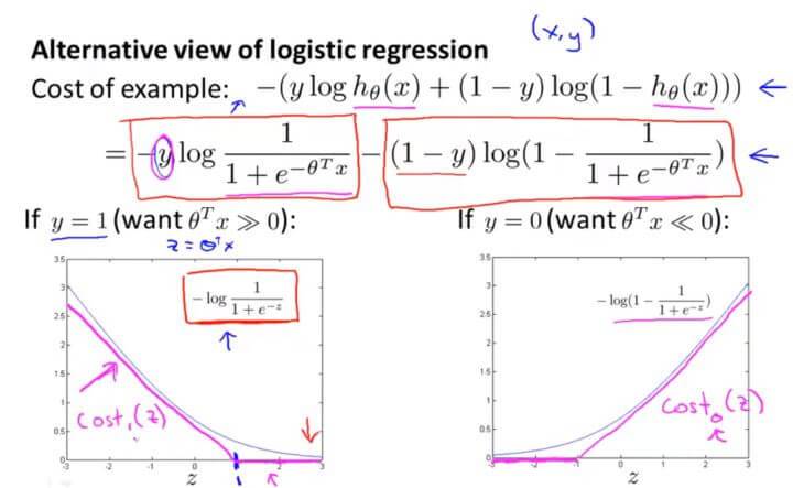
When y=1, as the value of z increases, the prediction cost decreases. Therefore, when logistic regression faces a positive sample y=1 and wants to achieve sufficiently high prediction accuracy, it wants $z= \theta^Tx\gg 0 $ . SVM, however, straightens the curve in the figure above into the piecewise linear curve in the figure below, forming the cost-function curve $cost_1(z)$ when y=1:
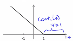
When y=1, to make the prediction accuracy sufficiently high, SVM wants $\theta^Tx\geqslant 1$ .
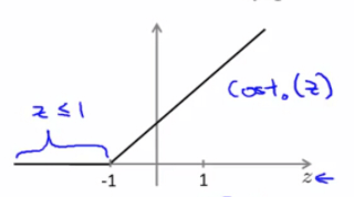
Similarly, when y=0, SVM defines the cost function $cost_0(z)$ . To make the prediction accuracy sufficiently high, SVM wants $\theta^Tx \leqslant -1$ :
In logistic regression, the cost function is:
$$J(\theta)=min_{\theta} \frac{1}{m}[\sum_{i=1}^{m}{y^{(i)}}(-logh_\theta(x^{(i)}))+(1-y^{(i)})((-log(1-h_\theta(x^{(i)})))]+\frac{\lambda}{2m}\sum_{j=1}^{n}{\theta_j^2}$$
For logistic regression, its cost function is determined by two terms. The first term is the cost from the training samples, and the second term is the regularization term. This is equivalent to minimizing A plus the regularization parameter $\lambda$ multiplied by the squared-parameter term B; its form is roughly: $A+\lambda B$ . Here we achieve optimization by setting different regularization parameters $\lambda$ . But in support vector machines, the parameter is moved to the front, using the parameter C as the coefficient of A and taking A as the weighted term. So its form is: $CA+B$ .
In logistic regression, we adjust the relative weights of A and B through the regularization parameter $\lambda$ , and the weight of A is inversely proportional to the value of $\lambda$ . In SVM, we adjust the relative weights of A and B through the parameter C, and the weight of A is proportional to the value of C. In other words, the parameter C can be viewed as playing the role of $\frac{1}{\lambda}$ .
Therefore, the term $\frac{1}{ m}$ is merely a constant and has no effect at all on minimizing the parameter $\theta$ , so we remove it here.
The cost function of a support vector machine is:
$$min_{\theta} C[\sum_{i=1}^{m}{y^{(i)}}cost_1(\theta^Tx^{(i)})+(1-y^{(i)})cost_0(\theta^Tx^{(i)})]+\frac{1}{2}\sum_{j=1}^{n}{\theta_j^2}$$
Unlike logistic regression, whose hypothesis function outputs a probability, a support vector machine directly predicts whether the value of y is 0 or 1. In other words, its hypothesis function looks like this:
$$h_{\theta}(x)=\left{\begin{matrix} 1,;;if; \theta^{T}x\geqslant 0\ 0,;;otherwise \end{matrix}\right.$$
II. Large Margin Classification: Large-Margin Classifier
A support vector machine is the last supervised learning algorithm. Compared with the logistic regression and neural networks we studied earlier, support vector machines provide a clearer and more powerful approach for learning complex nonlinear equations.
Support vector machines are also called large margin classifiers.
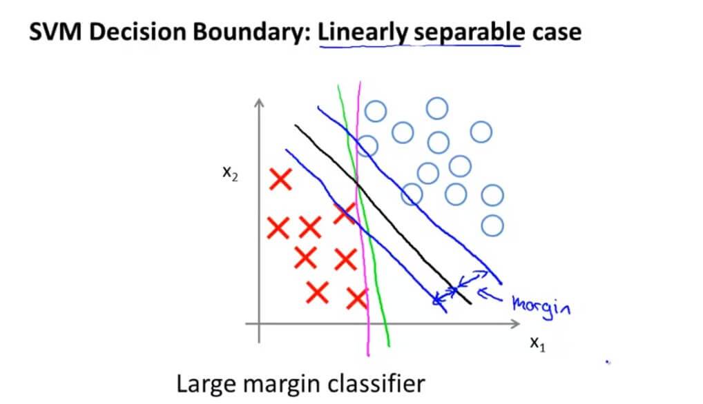
Suppose we have a dataset like this. We can see that it is linearly separable. However, sometimes our decision boundary may look like the green line or the pink line in the figure; neither of these decision boundaries seems like a particularly good choice. A support vector machine will choose the black decision boundary. Compared with the previous ones, the black boundary has a larger distance from both positive and negative samples, and this distance is called the margin. This is also why we call support vector machines large-margin classifiers.
The support vector machine model works by trying to separate positive and negative samples with the largest possible margin.
$$min_{\theta} C[\sum_{i=1}^{m}{y^{(i)}}cost_1(\theta^Tx^{(i)})+(1-y^{(i)})cost_0(\theta^Tx^{(i)})]+\frac{1}{2}\sum_{j=1}^{n}{\theta_j^2}$$
When y=1, SVM wants $\theta^Tx\geqslant 1$ . When y=0, SVM wants $\theta^Tx \leqslant -1$ . For the preceding term A in the cost function, the ideal minimum is, of course, 0. So this becomes:
$$min_{\theta}\frac{1}{2}\sum_{i=1}^{n}{\theta_j^2};;;;;; \left{\begin{matrix}
\theta^Tx\geqslant 1,if ;y^{(i)}=1 \
\theta^Tx\leqslant 1 ,if ;y^{(i)}=0
\end{matrix}\right.
$$
Derivation
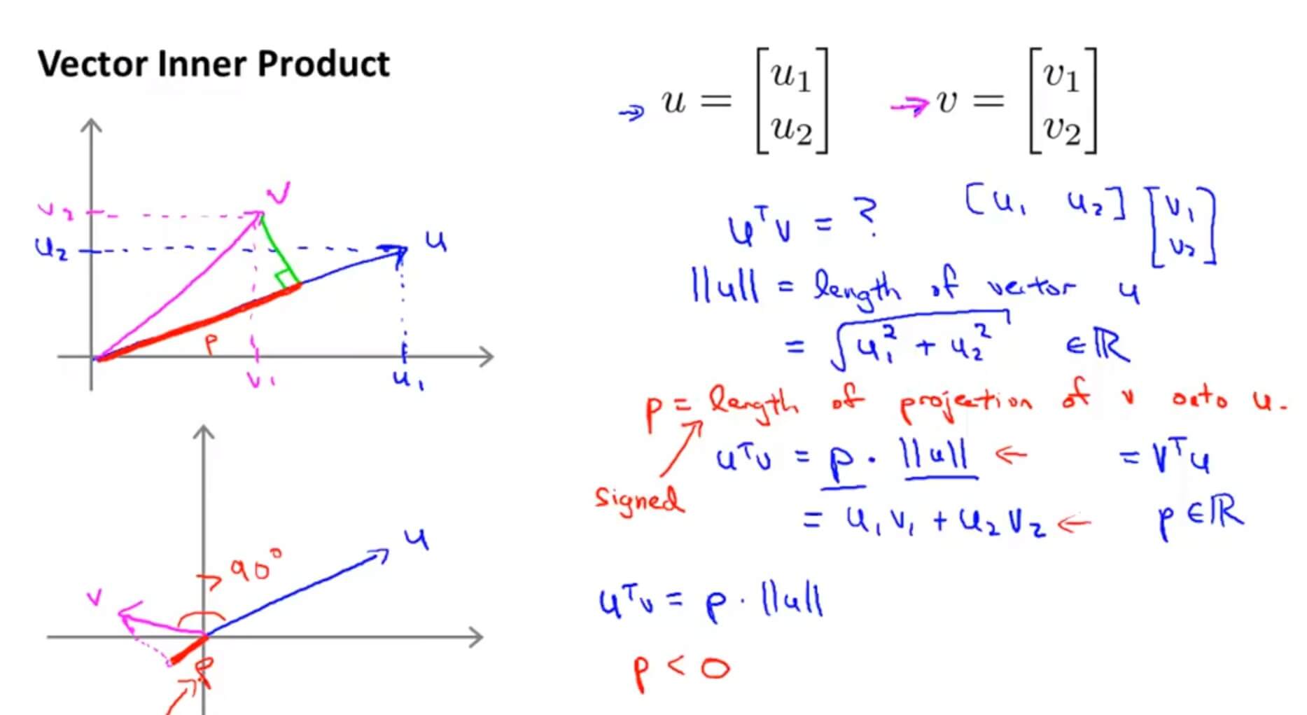
Taking two two-dimensional vectors as an example, we project vector v onto vector u. The length of the projection is p, and $\left | u \right |$ is the magnitude of vector u. Then the inner product of the vectors is equal to $p*\left | u \right |$ . In algebra, the vector inner product can be expressed as: $u_1v_1+u_2v_2$ . From this definition, we can obtain: $u^Tv=u_1v_1+u_2v_2$ .
$\left | u \right |$ is the norm of $\overrightarrow{u}$ , that is, the Euclidean length of vector $\overrightarrow{u}$ .
The minimization function is: $$min_{\theta}\frac{1}{2}\sum_{i=1}^{n}{\theta_j^2}$$
Here we use a simple two-dimensional example:
$$min_{\theta}\frac{1}{2}\sum_{i=1}^{n}{\theta_j^2}=\frac{1}{2}(\theta_1^2+\theta_2^2)=\frac{1}{2}(\sqrt{\theta_1^2+\theta_2^2})^2=\frac{1}{2}\left | \theta \right |^2$$
Pythagorean theorem:
$$ \left | u \right | = \sqrt{u_{1}^{2} + u_{2}^{2}}$$
As long as $\theta$ can be minimized, the minimization function can attain its minimum.
When it is perpendicular, $\theta$ takes its minimum value. This explains why the decision boundary of a support vector machine would not choose the green line in the left figure. For ease of understanding, let $\theta_0=0$ , which means the decision boundary must pass through the origin. Then we can see the relationship between $\theta $ and $x^{(i)}$ perpendicular to the decision boundary (the red projection and the pink projection). We can see that the values of their projections $p^{(i)}$ are both relatively small, which also means that the value of $||\theta||^2$ must be large. This is obviously in conflict with the minimization objective $\frac{1}{2}||\theta||^2$ . Therefore, the decision boundary of a support vector machine will make the projection of $p^{(i)}$ onto $\theta$ as large as possible. This is why the decision boundary is the one shown in the right figure, and also why support vector machines can effectively produce maximum-margin classification.
III. Kernels
1. Definition
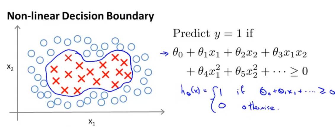
Previously, when we fit a nonlinear decision boundary to distinguish positive and negative samples, we constructed polynomial feature variables.
First, let’s use a new notation to represent the decision boundary: $\theta_0+\theta_1f_1+\theta_2f_2+\theta_3f_3+\cdots $ . Here we use $f_i$ to represent new feature variables.
If it were the decision boundary we learned earlier, then it would be: $f_1=x_1 , f_2=x_2 , f_3=x_1x_2 , f_4=x_1^2 , f_5=x_2^2$ , and so on. But using such high-order terms as feature variables is not necessarily what we need, and the computational cost is enormous. So are there any other higher-level feature variables?
Below is one idea for constructing new features:
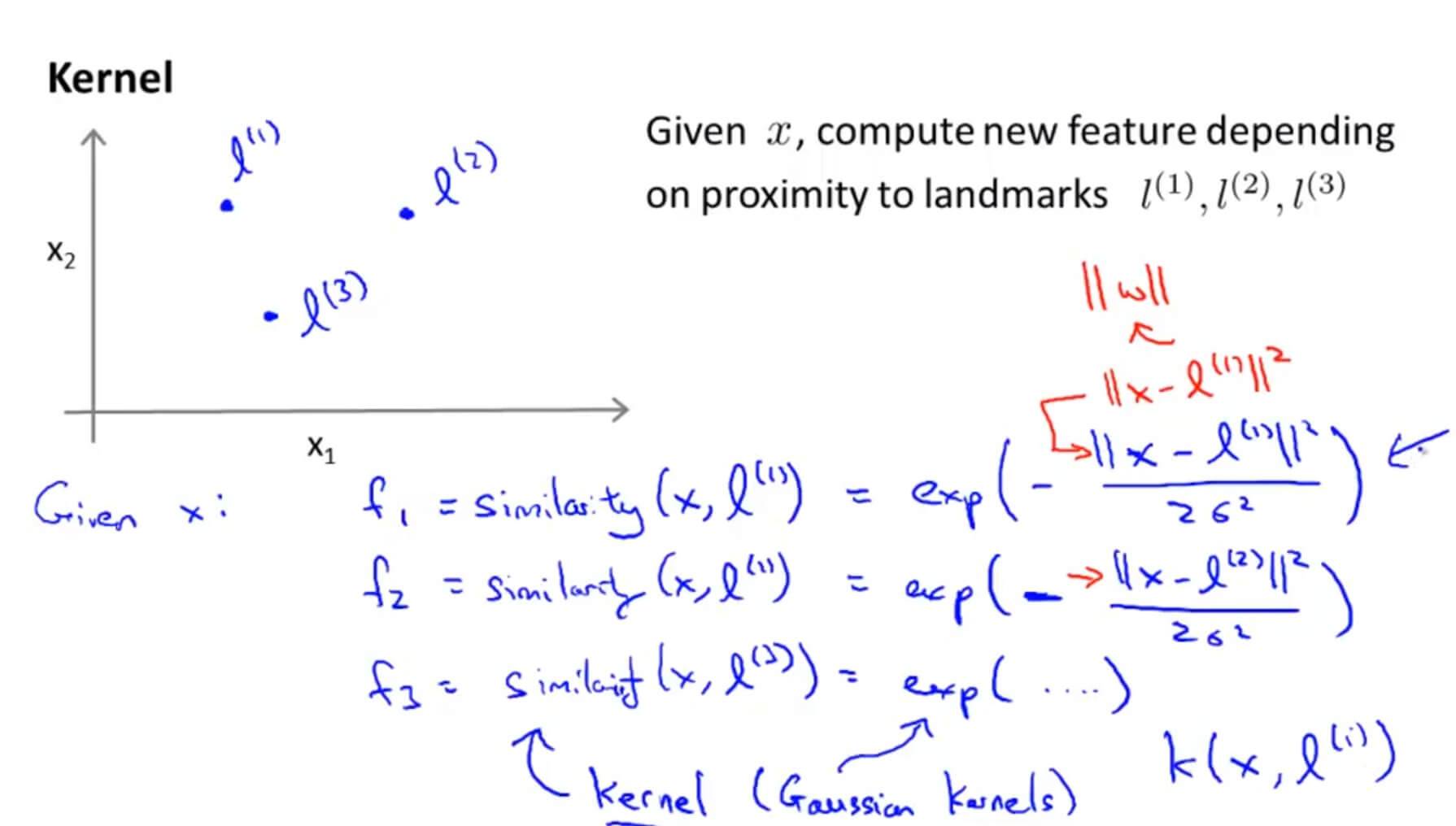 For simplicity, we define only three feature variables here. First, we manually select three different points on the $x_1,x_2$ coordinate axes: $l^{(1)},l^{(2)},l^{(3)}$.
Then we define the first feature as: $f_1=similarity(x,l^{(1)})$, which can be interpreted as the similarity between sample x and the first landmark $l^{(1)}$. This relationship can be expressed with the following formula: $f_1=similarity(x,l^{(1)})=exp(-\frac{||x-l^{(1)}||^2}{2\sigma^2})$ (exp: the exponential function with the natural constant e as the base)
Similarly: $f_2=similarity(x,l^{(2)})=exp(-\frac{||x-l^{(2)}||^2}{2\sigma^2})$,
$f_3=similarity(x,l^{(3)})=exp(-\frac{||x-l^{(3)}||^2}{2\sigma^2})$. We call this expression a kernel function (Kernels). Here, the kernel function we choose is the Gaussian kernel (Gaussian Kernels).
So what is the relationship between the Gaussian kernel and similarity?
First look at the first feature $f_1$: $f_1=similarity(x,l^{(1)})=exp(-\frac{||x-l^{(1)}||^2}{2\sigma^2})=exp(\frac{\sum_{j=1}^{n}{(x_j-l_j^{(1)})^2}}{2\sigma^2})$
If sample x is very close to $l^{(1)}$, i.e. $x\approx l^{(1)}$, then: $ f_1\approx exp(-\frac{0^2}{2\sigma^2})\approx 1$.
If sample x is very far from $l^{(1)}$, i.e. $x\gg l^{(1)}$, then: $ f_1\approx exp(-\frac{\infty^2}{2\sigma^2})\approx 0$.
The visualization is as follows:
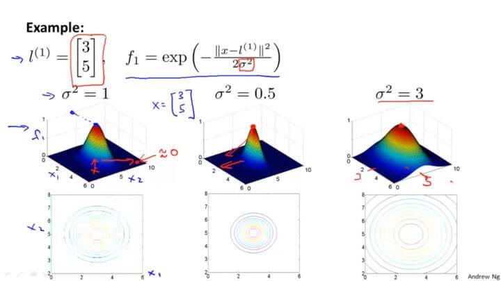
As can be seen from the figure, the closer it is to $l^{(1)} , f_1$, the larger the value.
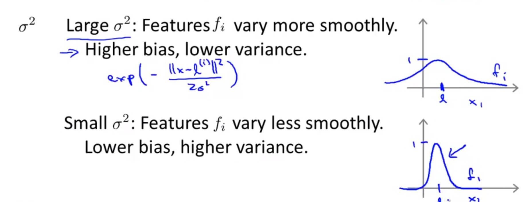
As an aside, let’s talk about how the Gaussian kernel parameter $\sigma^2$ affects the function. As can be seen from the figure, decreasing or increasing it only affects how wide or narrow the curve is; in other words, it affects only the rate at which the value increases or decreases.
2. Landmark Selection
Using landmarks and kernel functions, we can train very complex nonlinear decision boundaries. So where do the landmarks $l^{(1)},l^{(2)},l^{(3)}$ come from?
Assume we have the following dataset:
$$(x^{(1)},y^{(1)}),(x^{(2)},y^{(2)}),(x^{(3)},y^{(3)})\cdots(x^{(m)},y^{(m)})$$
We take each sample as a landmark:
$$l^{(1)}=x^{(1)},l^{(2)}=x^{(2)},l^{(3)}=x^{(3)}\cdots l^{(m)}=x^{(m)}$$
Then for sample $(x^{(i)},y^{(i)})$, we compute its distance to each landmark:
$$
\begin{matrix}
f^{(i)}_1=sim(x^{(i)},l^{(1)})\
f^{(i)}_2=sim(x^{(i)},l^{(2)})\
\vdots \
f^{(i)}_m=sim(x^{(i)},l^{(3)})\
\end{matrix}
$$
This gives the new feature vector: $f \in \mathbb{R}^{m+1} $
$$f = \begin{bmatrix} f_0\ f_1\ f_2\ \vdots \ f_m \end{bmatrix} $$
where $f_0=1$
The training process for an SVM with a kernel function is therefore as follows:
$$min_{\theta} C[\sum_{i=1}^{m}{y^{(i)}}cost_1(\theta^Tf^{(i)})+(1-y^{(i)})cost_0(\theta^Tf^{(i)})]+\frac{1}{2}\sum_{j=1}^{n}{\theta_j^2}$$
IV. SVMs in Practice
1. Using Popular Libraries
As one of today’s most popular classification algorithms, SVM already has many excellent implementation libraries, such as libsvm. Therefore, we no longer need to implement SVM manually ourselves (after all, an SVM model that can be used in production is not as simple as what is introduced in the course).
When using these libraries, we usually need to specify the two key components required by SVM:
- Parameter C
- Kernel function (Kernel)
Since C can be regarded as having the opposite effect of the regularization parameter $\lambda $, the tuning of C is as follows:
For low bias and high variance, i.e. when overfitting occurs: decrease the value of C.
For high bias and low variance, i.e. when underfitting occurs: increase the value of C.
For choosing a kernel function, here are some tips:
When the feature dimension n is high and the sample size m is small, it is not advisable to use a kernel function; otherwise, it can easily lead to overfitting.
When the feature dimension n is low and the sample size m is sufficiently large, consider using the Gaussian kernel. However, before using the Gaussian kernel, feature scaling is required.
When the kernel parameter $\sigma^2$ is large, the feature $f_i$ is relatively smooth; that is, the feature differences between samples become smaller. This causes underfitting (high bias, low variance), as shown in the upper figure below.
When $\sigma^2$ is small, the feature $f_i$ curve changes sharply; that is, the feature differences between samples become larger. This causes overfitting (low bias, high variance), as shown in the lower figure below:
2. Multiclass Classification
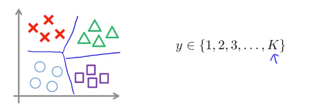
Usually, popular SVM libraries already have built-in APIs for multiclass classification. If multiclass classification is not supported, then, as with logistic regression, use the One-vs-All strategy for multiclass classification:
- Select one class i in turn and treat it as the positive class, i.e. class “1”; treat all remaining samples as negative samples, i.e. class “0”.
- Train the SVM to obtain parameters $\theta^{(1)},\theta^{(2)},\cdots,\theta^{(K)}$, i.e. obtain a total of K−1 decision boundaries.
3. Choosing a Classification Model
So far, the classification models we have learned are:
(1)Logistic regression;
(2)Neural networks;
(3)SVM
How should we choose among these three? We consider the feature dimension n and the sample size m:
If n is very large relative to m, for example n=10000 and $m\in(10,1000)$: choose logistic regression or an SVM without a kernel.
If n is relatively small and m is moderate, such as $n\in(1,1000)$ and $m\in(10,10000)$: choose an SVM with a Gaussian kernel.
If n is relatively small and m is large, such as $n\in(1,1000)$ and m>50000: at this point, create more features (for example, through polynomial expansion), and then use logistic regression or an SVM without a kernel. Neural networks adapt well to all of the above scenarios, but they are slower in terms of computational performance.
IV. Support_Vector_Machines Quiz
1. Question 1
Suppose you have trained an SVM classifier with a Gaussian kernel, and it learned the following decision boundary on the training set:

When you measure the SVM’s performance on a cross validation set, it does poorly. Should you try increasing or decreasing C? Increasing or decreasing $\sigma^{2}$?
A. It would be reasonable to try decreasing C. It would also be reasonable to try increasing $\sigma^{2}$.
B. It would be reasonable to try increasing C. It would also be reasonable to try increasing $\sigma^{2}$.
C. It would be reasonable to try increasing C. It would also be reasonable to try decreasing $\sigma^{2}$.
D. It would be reasonable to try decreasing C. It would also be reasonable to try decreasing $\sigma^{2}$.
Answer: A
For overfitting, you should decrease C and increase $\sigma^2$.
2. Question 2
The formula for the Gaussian kernel is given by similarity $(x,l^{(1)})=exp(-\frac{\left | x-l^{(1)} \right |^{2}}{2\sigma^{2} })$ .
The figure below shows a plot of f1=similarity $(x,l^{(1)})$ when $\sigma^{2} = 1$.

Which of the following is a plot of f1 when $\sigma^{2} = 0.25$?
A. 
B. 
C. 
D. 
Answer: A
When $\sigma^{2} $ becomes smaller, the curve becomes narrower and taller.
3. Question 3
The SVM solves
$$min_{\theta} C \sum^{m}_{i=1}y^{(i)}cost_{1}(\theta^{T}x^{(i)})+(1-y^{(i)})cost_{0}(\theta^{T}x^{(i)})+\sum^{n}_{j=1}\theta^{2}_{j}$$ where the functions $cost_0(z)$ and $cost_1(z)$ look like this:
The first term in the objective is:
$$C \sum^{m}{i=1}y^{(i)}cost{1}(\theta^{T} x^{(i)})+(1-y^{(i)})cost_{0}(\theta^{T}x^{(i)})$$
This first term will be zero if two of the following four conditions hold true. Which are the two conditions that would guarantee that this term equals zero?
A. For every example with $y^{(i)}=0$, we have that $\theta^{T}x(i) \leqslant 0$.
B. For every example with $y^{(i)}=1$, we have that $\theta^{T}x(i) \geqslant 0$.
C. For every example with $y^{(i)}=0$, we have that $\theta^{T}x(i)\leqslant-1$.
D. For every example with $y^{(i)}=1$, we have that $\theta^{T}x(i)\geqslant 1$.
Answer: C, D
4. Question 4
Suppose you have a dataset with n = 10 features and m = 5000 examples.
After training your logistic regression classifier with gradient descent, you find that it has underfit the training set and does not achieve the desired performance on the training or cross validation sets.
Which of the following might be promising steps to take? Check all that apply.
A. Try using a neural network with a large number of hidden units.
B. Create / add new polynomial features.
C. Reduce the number of examples in the training set.
D. Use a different optimization method since using gradient descent to train logistic regression might result in a local minimum.
Answer: A, B
The question asks how to address underfitting.
A. Increasing the number of hidden units in the neural network can help address underfitting.
B. Adding more features can help address underfitting.
C. Reducing the number of training examples will not work.
D. It is not the gradient descent function that reaches the minimum, but the cost function.
5. Question 5
Which of the following statements are true? Check all that apply.
A. Suppose you have 2D input examples (ie, $x^{(i)} \in \mathbb{R}^2$). The decision boundary of the SVM (with the linear kernel) is a straight line.
B. If the data are linearly separable, an SVM using a linear kernel will return the same parameters $\theta$ regardless of the chosen value of C (i.e., the resulting value of $\theta$ does not depend on C).
C. If you are training multi-class SVMs with the one-vs-all method, it is not possible to use a kernel.
D. The maximum value of the Gaussian kernel (i.e., $sim(x,l^{(1)})$) is 1.
Answer: A, D
A. A linear decision boundary is a straight line.
B. $min_{\theta} C[\sum_{i=1}^{m}{y^{(i)}}cost_1(\theta^Tx^{(i)})+(1-y^{(i)})cost_0(\theta^Tx^{(i)})]+\frac{1}{2}\sum_{j=1}^{n}{\theta_j^2}$; $\theta$ is precisely determined by the value of C.
C. SVMs can be used to solve multi-class classification problems.
D. The range of the Gaussian kernel function is: [0,1].
GitHub Repo: Halfrost-Field
Follow: halfrost · GitHub